Map across resamples

fit_resamples() and tune_grid() are tidymodels functions that we use in combination with objects generated from a resampling function (e.g., vfold_cv(), bootstraps(), etc from the rsample package) to get held-out performance estimates for our models.

fit_resamples() and tune_grid() use looping under the hood to accomplish their goals. fit_resamples() loops over the splits generated by our resampling function to get held-out performance estiamtes for a single model configuration.
tune_grid() also loops over these splits but includes an additional inner loop that loops over the values of our hyper-parameters in a hyper-parameter grid that we create.

In this appendix, we are going to re-create the functionality of fit_resamples() and tune_grid() using the map() function from the purrr package. This will help us understand how these functions work under the hood and give us a better understanding of how to use them. It will also give us an alternative way to do resampling if we need it.

Specifically, with respect to using resampling to get held-out performance estimates, we will

Gain a better understanding of the resampling object that is returns from bootstraps() and vfold_cv()
Make more transparent how these functions incorporate loops as part of their computations
Be able to reproduce these computations, manually for when we can’t use these functions directly.
- This might be if we want to loop over model configurations that are not defined by differece in hyperparameters but instead by other characteristics (e.g., different recipes, different statistical algorithms).
- We want to use an algorigthm that is not supported by tidymodels (e.g., we are developing deep neural networks outside of tidymodels by directly using the keras package)
We want to do nested resampling (e.g., using bootstraps() to both select a best model configuration and evaluate that best configuration with the variance benefits that are offered by nested cv relative to using a single held out test set.

More generally, we will also gain a better understanding (and some code examples) of the use of list columns with iteration via map().

This has many other uses than just resampling.
Wickham has writting about this in more detail elsewhere.

In this appendix, we will work through four separate examples that build in complexity

First, we will reproduce fit_resamples() computations by using map() to loop over the splits and fit a single model to each split. We use separate independent maps() for each step
Next, we will do this again but by wrapping all the steps into one function and using a single call to map() to loop that function over the splits.
The third example, will reproduce tune_grid() by using two nested map()s to loop over the splits and the hyper-parameter grid.
The final example will demonstrate how to do nested resampling using map() Nested resampling includes both an outer and inner loop across different out and inner splits. There is also an innermost loop across values in a hyper-parameter grid (or any other grid that defines different model configurations)

Set up

Lets start all of these examples by….

Loading libraries

Code

library(tidyverse)
library(tidymodels)

Creating a simple data set that has 300 observationns and two predictors (x1 and x2) and one outcome (y). The outcome is a linear combination of the two predictors with some noise added.

Code

set.seed(123456)
n_obs <- 300
d <- tibble(x1 = rnorm(n_obs), x2 = rnorm(n_obs), y = 2*x1 + 3*x2 + rnorm(n_obs))

Getting bootstrap resamples of d.

Code

n_boots <- 50
resamples <- bootstraps(d, times = n_boots)

bootstraps()

Returns an object that two columns and n_boots (in this case 50) rows. Each row is a bootstrap sample of the data. The columns are:
splits - contains a bootstrap sample of the data that includes held-in raw data and OOB held-out raw data subsamples
id - name of the resample

Code

resamples

# Bootstrap sampling 
# A tibble: 50 × 2
   splits            id         
   <list>            <chr>      
 1 <split [300/115]> Bootstrap01
 2 <split [300/108]> Bootstrap02
 3 <split [300/108]> Bootstrap03
 4 <split [300/107]> Bootstrap04
 5 <split [300/112]> Bootstrap05
 6 <split [300/102]> Bootstrap06
 7 <split [300/112]> Bootstrap07
 8 <split [300/114]> Bootstrap08
 9 <split [300/115]> Bootstrap09
10 <split [300/117]> Bootstrap10
# ℹ 40 more rows

This resamples object is a tibble (as typical in the tidy framework).

However, it uses “list columns” to hold the splits.
In a typical tibble, the individual cells in any column contain numeric or character data. However, this is not required. A column in a tibble is just a list and therefore, the cells can contain any type of object.
The cells for the splits column in this tibble contain splits, a special object created by functions in the rsample package that hold resampled datasets.

We can extract the contents of one of these cells using the base R [[]] notation

The first resample used the full 300 observations from d (the last value)
It make a bootstrap resample of 300 observations from d (the first value) that we can use as held-in data for training models
There are 115 OOB observations for this split that we can use as held-out data

Code

resamples$splits[[1]]

<Analysis/Assess/Total>
<300/115/300>

We will also need a recipe to create features from our raw data. Here is a simple recipe that indicate that y will be models on all the other columns (x1 and x2). We will not do any other feature engineering to keep this example simple.

Code

rec <- recipe(y ~ ., data = d)

We are now ready to start the first example

Using map() to replace fit_resamples() - step x step

In this first example, we will combine map() with the use of list columns to save all the intermediate products that are produced when fitting and evaluating a single model configuration for a simple linear regression across many (in this case 50) held-out sets created by bootstrapping.

To do this, we will need a function to fit linear models to held-in training data. We can use the typical tidymodels code here.

Code

fit_lm <- function(held_in) {
  linear_reg() |> 
    set_engine("lm") |> 
    fit(y ~ ., data = held_in)
}

Then we use map() and list columns to save the individual steps for evaluating the model in each split/resample. The following steps are done for EACH resample using map() or map2()

Prep the recipe with held-in data (in prep_recs column)
Bake the recipe using new_data = NULL to get held-in features (in held_ins)
Bake the recipe using new_data = assessment(split) to get held-out features (in held_outs)
Fit the model using the held-in features (in models)
Get predictions using the model with the held-out features (in predictions)
Calculate the rmse of the model (in rmses)

Code

resamples_ex1 <- resamples |> 
  mutate(prep_recs = map(splits, 
                         \(split) prep(rec, training = analysis(split))),
         held_ins = map2(resamples$splits, prep_recs, 
                         \(split, prep_rec) bake(prep_rec, new_data = NULL)),
         held_outs = map2(resamples$splits, prep_recs, 
                          \(split, prep_rec) bake(prep_rec, 
                                                  new_data = assessment(split))),
         models = map(held_ins, 
                      \(held_in) fit_lm(held_in)),
         predictions = map2(models, held_outs, 
                            \(model, held_out) predict(model, held_out)$.pred),
         rmses = map2_dbl(predictions, held_outs, 
                           \(pred, held_out) rmse_vec(held_out$y, pred)))

The pipline above creates a tibble with columns for each of the intermediate products and the rmse/error of the model in each resample.

All but the last columns are list columns that can hold objects of any time (e.g., prepped recipes, data frames, model objects).
The final column is a double column that holds the numeric rmse of the model in each resample. That is why we used map_dbl() to create the rmses column.

Code

resamples_ex1 |> glimpse()

Rows: 50
Columns: 8
$ splits      <list> [<boot_split[300 x 115 x 300 x 3]>], [<boot_split[300 x 1…
$ id          <chr> "Bootstrap01", "Bootstrap02", "Bootstrap03", "Bootstrap04"…
$ prep_recs   <list> [x1, x2, y, double, numeric, double, numeric, double, num…
$ held_ins    <list> [<tbl_df[300 x 3]>], [<tbl_df[300 x 3]>], [<tbl_df[300 x …
$ held_outs   <list> [<tbl_df[115 x 3]>], [<tbl_df[108 x 3]>], [<tbl_df[108 x …
$ models      <list> [NULL, ~NULL, ~NULL, regression, FALSE, stats, formula, f…
$ predictions <list> <1.38587470, 2.84334628, -2.07435584, 1.24941793, -0.0569…
$ rmses       <dbl> 0.9826968, 0.9380291, 1.0127994, 0.9929520, 0.9849202, 0.9…

We can now look at rmses across the 50 bootstraps. For example, we can make a histogram using ggplot from the errors column in the fits tibble

Code

resamples_ex1 |> 
  ggplot(aes(rmses)) +
  geom_histogram(binwidth = 0.05)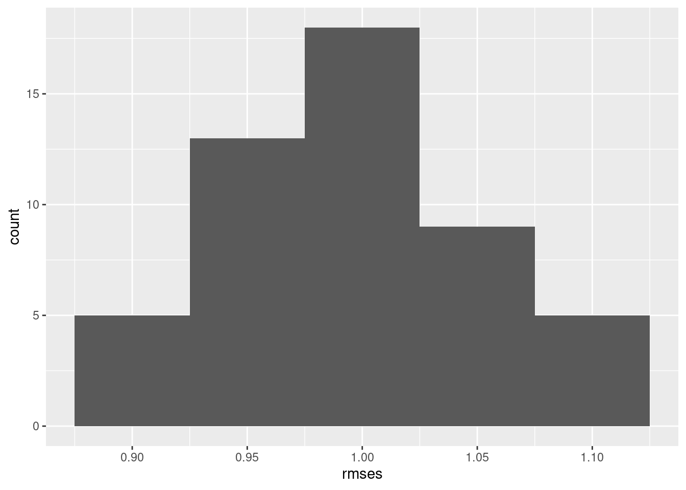

And we can summarize the min, max, mean, median and stdev of the error column in the fits tibble

Code

resamples_ex1 |> 
  summarize(n = n(),
            min = min(rmses), 
            max = max(rmses), 
            mean = mean(rmses), 
            median = median(rmses),
            std_dev = sd(rmses))

# A tibble: 1 × 6
      n   min   max  mean median std_dev
  <int> <dbl> <dbl> <dbl>  <dbl>   <dbl>
1    50 0.876  1.12 0.997  0.989  0.0557

Easy peasy!

This first example has demonstrated the use of map() and list columns, which has many uses.
This first example also makes clear what fit_resamples() is doing.
It also gives you an alternative workflow in case you can’t use fit_resamples().
- This might occur if you are training deep neural networks with keras directly.
- In that instance, you might use the fit() function from keras to fit the model and then use predict() to get predictions. But you could still use the functions from the rsample package to get a resampled object (e.g., using bootstraps()) and you could use performance metrics (e.g., rmse_vec()) from the yardstick package.

But remember, if you can (and in most instances, you can), it is easier to still using fit_resamples() to get your held-out performance estimates.

Code

resamples_tidy_ex1 <-
  linear_reg() |> 
    set_engine("lm") |> 
    fit_resamples(preprocessor = rec, 
                  resamples = resamples, 
                  metrics = metric_set(rmse))

resamples_tidy_ex1 |> 
  collect_metrics()

# A tibble: 1 × 6
  .metric .estimator  mean     n std_err .config             
  <chr>   <chr>      <dbl> <int>   <dbl> <chr>               
1 rmse    standard   0.997    50 0.00788 Preprocessor1_Model1

Code

resamples_tidy_ex1 |> 
  collect_metrics(summarize = FALSE)

# A tibble: 50 × 5
   id          .metric .estimator .estimate .config             
   <chr>       <chr>   <chr>          <dbl> <chr>               
 1 Bootstrap01 rmse    standard       0.983 Preprocessor1_Model1
 2 Bootstrap02 rmse    standard       0.938 Preprocessor1_Model1
 3 Bootstrap03 rmse    standard       1.01  Preprocessor1_Model1
 4 Bootstrap04 rmse    standard       0.993 Preprocessor1_Model1
 5 Bootstrap05 rmse    standard       0.985 Preprocessor1_Model1
 6 Bootstrap06 rmse    standard       0.947 Preprocessor1_Model1
 7 Bootstrap07 rmse    standard       1.00  Preprocessor1_Model1
 8 Bootstrap08 rmse    standard       1.06  Preprocessor1_Model1
 9 Bootstrap09 rmse    standard       1.05  Preprocessor1_Model1
10 Bootstrap10 rmse    standard       0.981 Preprocessor1_Model1
# ℹ 40 more rows

Using map() to replace fit_resamples() - one function

If we wanted to generate the held-out error using resampling but didnt need/want the intermediate products, we could wrap all the steps in one function and just map that single function.

We might do this if we are working with big datasets and saving all the intermediate products requires too much memory.
Of course, we could also blend the this example with the previous example to save some but not all the intermediate products.

Here is a function that takes a split and a recipe and returns the rmse of the model fit to the held-in data and evaluated on the held-out data. It does all the steps we did in the previous example but in one function. We will use this function to replace all the intermediate steps in the previous example.

Code

fit_and_eval <- function(split, rec) {
  # prep the recipe with held-in data
  prep_rec <- prep(rec, training = analysis(split))
  
  # bake the recipe using new_data = NULL to pull out the held-in features
  held_in <- bake(prep_rec, new_data = NULL)
  
  # bake the recipe using new_data = assessment(split) to get held-out features
  held_out <- bake(prep_rec, new_data = assessment(split))
  
  # fit the model using the held-in features
  model <- 
    linear_reg() |> 
    set_engine("lm") |> 
    fit(y ~ ., data = held_in)
  
  # get predictions using the model with the held-out features
  pred <- predict(model, held_out)$.pred
  
  # calculate the accuracy of the model
  rmse_vec(held_out$y, pred)
}

Now map this function over the splits to get a vector of rmse. Same results, but not saving intermediate steps by using one function.

Code

resamples_ex2 <- resamples |> 
  mutate(errors = map_dbl(splits, \(split) fit_and_eval(split, rec)))

Here is what the resamples_ex2 tibble now looks like

Code

resamples_ex2

# Bootstrap sampling 
# A tibble: 50 × 3
   splits            id          errors
   <list>            <chr>        <dbl>
 1 <split [300/115]> Bootstrap01  0.983
 2 <split [300/108]> Bootstrap02  0.938
 3 <split [300/108]> Bootstrap03  1.01 
 4 <split [300/107]> Bootstrap04  0.993
 5 <split [300/112]> Bootstrap05  0.985
 6 <split [300/102]> Bootstrap06  0.947
 7 <split [300/112]> Bootstrap07  1.00 
 8 <split [300/114]> Bootstrap08  1.06 
 9 <split [300/115]> Bootstrap09  1.05 
10 <split [300/117]> Bootstrap10  0.981
# ℹ 40 more rows

And here we demo getting overall held-out performance details across the 50 bootstraps.

Code

resamples_ex2 |> 
  summarize(n = n(),
            min = min(errors), 
            max = max(errors), 
            mean = mean(errors), 
            median = median(errors),
            std_dev = sd(errors))

# A tibble: 1 × 6
      n   min   max  mean median std_dev
  <int> <dbl> <dbl> <dbl>  <dbl>   <dbl>
1    50 0.876  1.12 0.997  0.989  0.0557

Using two map()s to replace tune_grid()

Now we can make this a bit more complicated by adding a grid of hyperparameters to tune.

Lets keep it simple and tune only k in a knn model.
To tune k, we would normally use tune_grid() but we can do it again with two loops using map().
We use an outer map() to loop over the resamples (as we did in the last two examples) and an inner map() to loop over the values of k

Lets start by setting up a grid of values of k to tune over.

Code

grid_k = tibble(neighbors = c(3, 6, 9, 12, 15, 18))

We will use a single function to repeatedly fit and eval over our grid of parameters.

Code

eval_grid <- function(split, rec, grid_k) {
 
  # get held-in and held-out features for split 
  # we calculate features inside the function where we fit all models across the grid 
  # because we want to make sure we only need to prep and bake the recipe once
  # per split.  Otherwise, we would waste a lot of computational time.
  prep_rec <- prep(rec, training = analysis(split))
  held_in <- bake(prep_rec, new_data = NULL)
  held_out <- bake(prep_rec, new_data = assessment(split))

  # function to fit and eval model for a specific k using held-in/held-out
  # for this split
  fit_eval <- function(k, held_in, held_out) {
    model <- 
      nearest_neighbor(neighbors = k) |>   
        set_engine("kknn") |>   
        set_mode("regression") |>  
        fit(y ~ ., data = held_in)
    
    pred <- predict(model, held_out)$.pred
   
    # lets put k and rmse in a tibble and return that for each split 
    tibble(k = k, 
           rmse = rmse_vec(held_out$y, pred))
  }
  
  # loop through grid_k and fit/eval model for each k 
  # this is the inner loop from tune_grid()
  # use list_rbind() to bind the separate rows for each tibble into one larger tibble
  grid_k$neighbors |> 
    map(\(k) fit_eval(k, held_in, held_out)) |> 
    list_rbind()
}

Now we map this function over the 50 bootstrap splits.

This is the outer loop from tune_grid().
eval_grid() will return a tibble with rows for each value of k. We will save one tibble for each split in a list column called `rmses``.

Code

resamples_ex3 <- resamples |> 
  mutate(rmses = map(splits, 
              \(split) eval_grid(split, rec, grid_k)))

The rmses column contains the rmse for each value of k for each split/resample in a tibble. Each tibble has 6 rows (one for each k) and 2 columns (k and rmse).

Code

resamples_ex3

# Bootstrap sampling 
# A tibble: 50 × 3
   splits            id          rmses           
   <list>            <chr>       <list>          
 1 <split [300/115]> Bootstrap01 <tibble [6 × 2]>
 2 <split [300/108]> Bootstrap02 <tibble [6 × 2]>
 3 <split [300/108]> Bootstrap03 <tibble [6 × 2]>
 4 <split [300/107]> Bootstrap04 <tibble [6 × 2]>
 5 <split [300/112]> Bootstrap05 <tibble [6 × 2]>
 6 <split [300/102]> Bootstrap06 <tibble [6 × 2]>
 7 <split [300/112]> Bootstrap07 <tibble [6 × 2]>
 8 <split [300/114]> Bootstrap08 <tibble [6 × 2]>
 9 <split [300/115]> Bootstrap09 <tibble [6 × 2]>
10 <split [300/117]> Bootstrap10 <tibble [6 × 2]>
# ℹ 40 more rows

Lets take a look at one of these tibbles to make this structure clearer. The same tibble format is saved for all fifty bootstrap splits (with different values for rmse of course!)

Code

resamples_ex3$rmses[[1]]

# A tibble: 6 × 2
      k  rmse
  <dbl> <dbl>
1     3  1.51
2     6  1.47
3     9  1.47
4    12  1.52
5    15  1.56
6    18  1.61

We can unnest() the rmses column to get a tibble with one row for each k value in each resample.

unnest() is used frequently when a list column contains tibbles and you want to combine those tibbles into more traditional tibble without the list column.
No need to display the original splits column so we will select it out.

Code

resamples_ex3 |> 
  unnest(rmses) |> 
  select(-splits) |>
  print(n = 30)

# A tibble: 300 × 3
   id              k  rmse
   <chr>       <dbl> <dbl>
 1 Bootstrap01     3  1.51
 2 Bootstrap01     6  1.47
 3 Bootstrap01     9  1.47
 4 Bootstrap01    12  1.52
 5 Bootstrap01    15  1.56
 6 Bootstrap01    18  1.61
 7 Bootstrap02     3  1.31
 8 Bootstrap02     6  1.25
 9 Bootstrap02     9  1.25
10 Bootstrap02    12  1.27
11 Bootstrap02    15  1.29
12 Bootstrap02    18  1.30
13 Bootstrap03     3  1.48
14 Bootstrap03     6  1.46
15 Bootstrap03     9  1.48
16 Bootstrap03    12  1.50
17 Bootstrap03    15  1.52
18 Bootstrap03    18  1.54
19 Bootstrap04     3  1.41
20 Bootstrap04     6  1.34
21 Bootstrap04     9  1.31
22 Bootstrap04    12  1.32
23 Bootstrap04    15  1.35
24 Bootstrap04    18  1.38
25 Bootstrap05     3  1.51
26 Bootstrap05     6  1.43
27 Bootstrap05     9  1.41
28 Bootstrap05    12  1.42
29 Bootstrap05    15  1.44
30 Bootstrap05    18  1.44
# ℹ 270 more rows

We can pipe this unnested tibble into a group_by() and summarize() to get the median (or mean) across resamples and then arrange to find the best k

Code

resamples_ex3 |> 
  unnest(rmses) |> 
  select(-splits) |>
  group_by(k) |> 
  summarize(n = n(),
            mean_rmse = mean(rmse)) |> 
  arrange(mean_rmse)

# A tibble: 6 × 3
      k     n mean_rmse
  <dbl> <int>     <dbl>
1     9    50      1.34
2    12    50      1.35
3     6    50      1.36
4    15    50      1.36
5    18    50      1.38
6     3    50      1.42

The example makes it clear that using resampling to tune a grid of hyperparameters is just a matter of looping over the resamples in an outer loop and looping over a grid of hyperparameters in an inner loop.

You might use this approach

if you wanted to select among model configurations that different by something other than hyper-parameters (e.g., different recipes, different statistical algorithms).
Or if you wanted to fit models not supported by tidymodels.

But of course, when you can use it, using tune_grid() is easier because it takes care of the nested looping internally.

Code

resamples_tidy_ex3 <- 
  nearest_neighbor(neighbors = tune()) |>   
    set_engine("kknn") |>   
    set_mode("regression") |>  
    tune_grid(preprocessor = rec, 
              resamples = resamples, 
              grid = grid_k, 
              metrics = metric_set(rmse))

resamples_tidy_ex3 |> 
  collect_metrics() |> 
  arrange(mean)

# A tibble: 6 × 7
  neighbors .metric .estimator  mean     n std_err .config             
      <dbl> <chr>   <chr>      <dbl> <int>   <dbl> <chr>               
1         9 rmse    standard    1.34    50  0.0184 Preprocessor1_Model3
2        12 rmse    standard    1.35    50  0.0202 Preprocessor1_Model4
3         6 rmse    standard    1.36    50  0.0165 Preprocessor1_Model2
4        15 rmse    standard    1.36    50  0.0216 Preprocessor1_Model5
5        18 rmse    standard    1.38    50  0.0225 Preprocessor1_Model6
6         3 rmse    standard    1.42    50  0.0161 Preprocessor1_Model1

Using map()s to do nested cv

Now lets do the most complicated version of this. Nested resampling involves looping over outer splits where the held out data are test sets used to evaluate best model configurations for each outer split and the inner loop makes validation sets that are used to select the best model configuration for each outer fold. However, if we are tuning a grid of hyperparameters, there is even a further nested loop inside the inner resampling loop to get performance metrics for each value of the hyperparameter in the validation sets.

rsample supports creating a nested resampling object.

You can specify different resampling for the inner and outer loops.
k-fold for the outer loop and bootstraps for the inner loop is a common choice.
However, neither fit_resamples() or tune_grid() support nested resampling. So we will always need to use nested map() to do this ourselves.

First, lets make the nested resampling object and explore it a bit

We will use 5-fold cv for the outer loop
We will use 10 bootstraps for the inner loop
These numbers were selected only to make the computations faster. You may need more splits.

Code

resamples_nested <- d |> 
  nested_cv(outside = vfold_cv(v = 5), inside = bootstraps(times = 10))

Lets take a look at it.

It has five rows for each of the five outer splits. The outer splits are the k-folds.
The inner_resamples column contains the inner splits associated with each outer k-fold split. Each inner split is a bootstrap resample with 10 bootstraps.

Code

resamples_nested

# Nested resampling:
#  outer: 5-fold cross-validation
#  inner: Bootstrap sampling
# A tibble: 5 × 3
  splits           id    inner_resamples
  <list>           <chr> <list>         
1 <split [240/60]> Fold1 <boot [10 × 2]>
2 <split [240/60]> Fold2 <boot [10 × 2]>
3 <split [240/60]> Fold3 <boot [10 × 2]>
4 <split [240/60]> Fold4 <boot [10 × 2]>
5 <split [240/60]> Fold5 <boot [10 × 2]>

Lets look a little more carefully at this structure because its critical to understanding nested cv.

Below we pull out and look at the first outer k-fold split.
The total sample size is 300 and the outer k-fold split has 60 observations held-out to eventually use as a test set and 240 held-in that will eventually be used as training data when we train models in the outer loop to get our final performance metrics for best values of k. We will also use these held-in data in the inner loop.

Code

resamples_nested$splits[[1]]

<Analysis/Assess/Total>
<240/60/300>

Code

# I prefer to work with this resampled objects using base R notation
# however you could do the same using piped tidy code
# resamples_nested |> 
#   slice(1) |> 
#   pull(splits)

Now look below at the inner resamples for the first outer k-fold split.

For each outer k-fold split, we take the held-in data (240 observations in this case) and split it further, using the inner resampling method (10 bootstraps here).
Notice that each of the 10 bootstraps associated with the first outer k-fold split have 240 observation (because we used the held-in data from that outer k-fold split). These bootstrap resamples will be used as training data for the inner loop of nested. We will train models with various values of k with these data
Notice also that each of these 10 boostraps have held-out (OOB) observations that will be used as validation sets for the inner loop of nested. We will use these held-out validation sets to calculate performance metrics for the models with different value of k. This will let us select the best value of k for each outer split.

Code

resamples_nested$inner_resamples[[1]]

# Bootstrap sampling 
# A tibble: 10 × 2
   splits           id         
   <list>           <chr>      
 1 <split [240/87]> Bootstrap01
 2 <split [240/86]> Bootstrap02
 3 <split [240/80]> Bootstrap03
 4 <split [240/76]> Bootstrap04
 5 <split [240/89]> Bootstrap05
 6 <split [240/93]> Bootstrap06
 7 <split [240/90]> Bootstrap07
 8 <split [240/92]> Bootstrap08
 9 <split [240/93]> Bootstrap09
10 <split [240/87]> Bootstrap10

Now that we have a resamples object to use for nested cv, lets get some functions together to calculate rmses for inner validation sets and outer test sets

We will need a function again that takes a split, uses the recipe to get held-in/held-out features, and then fits and evaluates a model for each value of k in the grid. This is the exact same function as we used earlier (because we are using knn again). We include it below again for your review.

We will use this function twice.
In the inner loop of our nested cv, we will map this function over all 10 of our bootstraps associated with an outer split.
In the outer loop of our nested cv, we will map this function over all 5 of our outer splits using the best value of k that was identified for each outer split using its respective 10 bootstraps.

Code

eval_grid <- function(split, rec, grid_k) {
 
  # get held-in and held-out features for split 
  prep_rec <- prep(rec, training = analysis(split))
  held_in <- bake(prep_rec, new_data = NULL)
  held_out <- bake(prep_rec, new_data = assessment(split))

  # function fit fit and eval model for a specific lambda and resample
  fit_eval <- function(k, held_in, held_out) {
    model <- 
      nearest_neighbor(neighbors = k) |>   
        set_engine("kknn") |>   
        set_mode("regression") |>  
        fit(y ~ ., data = held_in)
    
    pred <- predict(model, held_out)$.pred
    
    # lets put k and rmse in a tibble and return that for each split 
    tibble(k = k, 
           rmse = rmse_vec(held_out$y, pred))
  }
  
  # loop through grid_k and fit/eval model for each k 
  # this is the inner loop
  # use list_rbind() to bind the separate rows for each tibble into one larger tibble
  grid_k$neighbors |> 
    map(\(k) fit_eval(k, held_in, held_out)) |> 
    list_rbind()
}

To loop eval_grid over the 10 bootstraps in the nested cv inner loop, we will need another simple function that applies our eval_grid() over each bootstrap within a set of 10 and binds the results into a single tibble.

Code

bind_bootstraps <- function(bootstraps, rec, grid_k) {
 
  bootstraps$splits |>  
    map(\(bootstrap_split) eval_grid(bootstrap_split, rec, grid_k)) |> 
    list_rbind()
}

Now we are ready to get performance metrics for each k in grid_k for each of the inner 10 bootstraps in each of the five outer k-folds splits. Remember that bind_bootstraps() just calls eval_grid() for each of the 10 bootstraps in the inner loop and binds the results.

Code

resamples_nested_ex4 <- resamples_nested |> 
  mutate(inner_rmses = map(inner_resamples, 
                          \(inner_resample) bind_bootstraps(inner_resample, 
                                                            rec, 
                                                            grid_k)))

Lets look at what we just added to our resamples object

We now have a tibble with 60 rows and 2 columns associated with each set of 10 inner bootstrap splits.

Code

resamples_nested_ex4

# Nested resampling:
#  outer: 5-fold cross-validation
#  inner: Bootstrap sampling
# A tibble: 5 × 4
  splits           id    inner_resamples inner_rmses      
  <list>           <chr> <list>          <list>           
1 <split [240/60]> Fold1 <boot [10 × 2]> <tibble [60 × 2]>
2 <split [240/60]> Fold2 <boot [10 × 2]> <tibble [60 × 2]>
3 <split [240/60]> Fold3 <boot [10 × 2]> <tibble [60 × 2]>
4 <split [240/60]> Fold4 <boot [10 × 2]> <tibble [60 × 2]>
5 <split [240/60]> Fold5 <boot [10 × 2]> <tibble [60 × 2]>

If we look at one of them, we see

The 60 rows are because we have 10 boostraps for each of the 6 values of k in the grid. So 10 * 6 = 60 rmses
we have columns for k and rmse

Code

resamples_nested_ex4$inner_rmses[[1]]

# A tibble: 60 × 2
       k  rmse
   <dbl> <dbl>
 1     3  1.52
 2     6  1.54
 3     9  1.58
 4    12  1.62
 5    15  1.65
 6    18  1.68
 7     3  1.77
 8     6  1.70
 9     9  1.69
10    12  1.70
# ℹ 50 more rows

We now need to calculate the best k for each of the sets of 10 boostraps (associated with one outer k-fold split). To do this, we average the 10 rmses together for each value of k and then choose the k with the lowest rmse. We will write a function to do this because we can then map that function over each of the sets of 10 bootstraps associated with each outer split.

Code

get_best_k <- function(rmses) {
  rmses |>  
    group_by(k) |> 
    summarize(mean_rmse = mean(rmse)) |> 
    arrange(mean_rmse) |> 
    slice(1) |> 
    pull(k)
}

And then map it across the sets of rmses for each outer k-fold splilt.

Code

resamples_nested_ex4 <- resamples_nested_ex4 |> 
  mutate(best_k = map_dbl(inner_rmses, \(rmses) get_best_k(rmses)))

Now we have determined the best value of k for each of the 5 outer folds.

Code

resamples_nested_ex4

# Nested resampling:
#  outer: 5-fold cross-validation
#  inner: Bootstrap sampling
# A tibble: 5 × 5
  splits           id    inner_resamples inner_rmses       best_k
  <list>           <chr> <list>          <list>             <dbl>
1 <split [240/60]> Fold1 <boot [10 × 2]> <tibble [60 × 2]>      6
2 <split [240/60]> Fold2 <boot [10 × 2]> <tibble [60 × 2]>     12
3 <split [240/60]> Fold3 <boot [10 × 2]> <tibble [60 × 2]>     12
4 <split [240/60]> Fold4 <boot [10 × 2]> <tibble [60 × 2]>      6
5 <split [240/60]> Fold5 <boot [10 × 2]> <tibble [60 × 2]>      9

We can now move up to the outer k-fold splits. We will use the best k for each outer fold to fit a model using the held-in data from the outer fold and then evaluate that model using the held-out test data. Those test data were NEVER used before so the will allow us to see how that model with a best value of k (selected by bootstrap resampling) performs in new data

We can reuse the eval_grid() function we used before to fit and evaluate the model using the held-in data and the held-out test data. But now we just use one value of k, the one that was best for each fold

Code

resamples_nested_ex4 <- resamples_nested_ex4 |> 
  mutate(test_rmse = map2(splits, best_k, 
                               \(split, k) eval_grid(split, rec, tibble(neighbors = k))))

We can pull the one row tibbles out of this final column and bind them together to get a tibble with one row for each outer fold. We have retained the best value of k for each fold for our information (these don’t need to be the same for each k-fold split).

Code

resamples_nested_ex4$test_rmse |> 
  list_rbind() |> 
  mutate(outer_fold = 1:length(resamples_nested_ex4$test_rmse)) |> 
  relocate(outer_fold)

# A tibble: 5 × 3
  outer_fold     k  rmse
       <int> <dbl> <dbl>
1          1     6  1.23
2          2    12  1.58
3          3    12  1.28
4          4     6  1.21
5          5     9  1.06

If we want to know the true best k to use when we train a final model to implement using all our data, we need select it by using our inner reasampling method (10 boostraps) with all our data.

We could then train our final implementation model by fitting a model to all our data using this value of k.

Final notes - parallel processing

All of these examples were done without the use of parallel processing. fit_resamples() and tune_grid() can use a parallel backend if you set it up.

You could modify our code to implement map() in parallel using future_map() from the furrr package.
For our fit_resamples() examples, there is only one map() or several independent ones. None are nested. Switch them all to future_map().
For our tune_grid() example, there are two nested maps(). In most instances, you will want to switch the outer loop map() to future_map() and leave the inner map() as is.
For our nested example, there are three nested map()s. In most instances, you will want to switch that outermost map() (across outer splits) to future_map() and leave the inner two map()s as is. - See our post on setting up parallel backends for more info on how to do that