Relative costs and benefits of these different statistical algorithms
4.2 Bayes Classifier
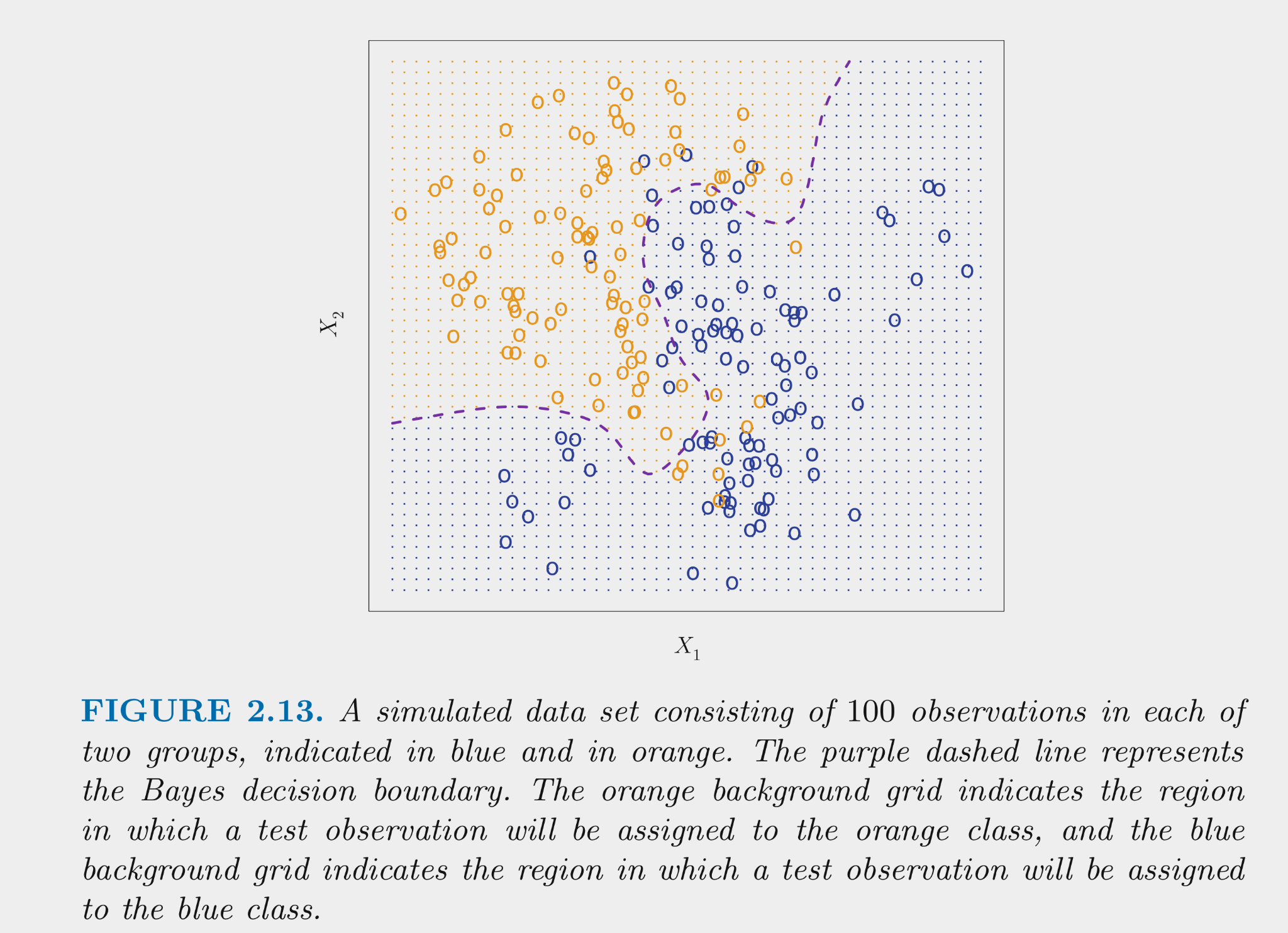
First, lets introduce the Bayes classifier, which is the classifier that will have the lowest error rate of all classifiers using the same set of features.
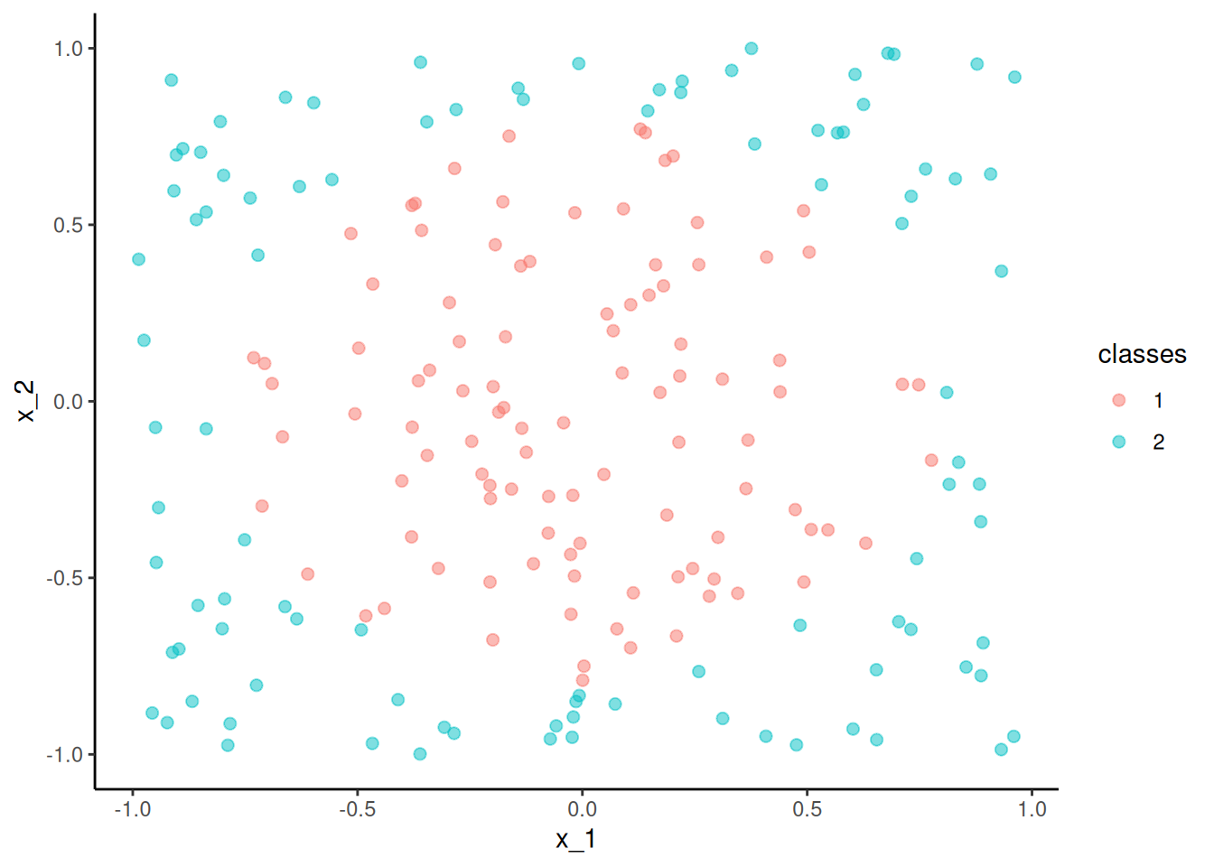
The figure below displays simulated data for a classification problem for K = 2 classes as a function of X1 and X2
The Bayes classifier assigns each observation its most likely class given its conditional probabilities for the values for X1 and X2
\(Pr(Y = k | X = x_0) for\:k = 1:K\)
For K = 2, this means assigning to the class with Pr > .50
This decision boundary for the two class problem is displayed in the figure
The Bayes classifier provides the minimum error rate for test data
Error rate for any \(x_0\) will be \(1 - max (Pr( Y = k | X = x_0))\)
Overall error rate will be the average of this across all possible X
This is the irreducible error for classification problems
This is a theoretical model b/c (except for simulated data), we don’t know the conditional probabilities based on X
Many classification models try to estimate these conditionals
Let’s talk now about some of these classification models
4.3 Logistic Regression: A Conceptual Review
Logistic regression (a special case of the generalized linear model) estimates the conditional probability for each class given X (a specific set of values for our features)
In the binary outcome case, we will often refer to the two outcomes as the positive class and the negative class
This makes most sense in some applied settings where we are most interested in predicting if one of the two classes is likely, e.g.,
Presence of heart disease
Positive for some psychiatric diagnoses
Lapse back to alcohol use in people with alcohol use disorder
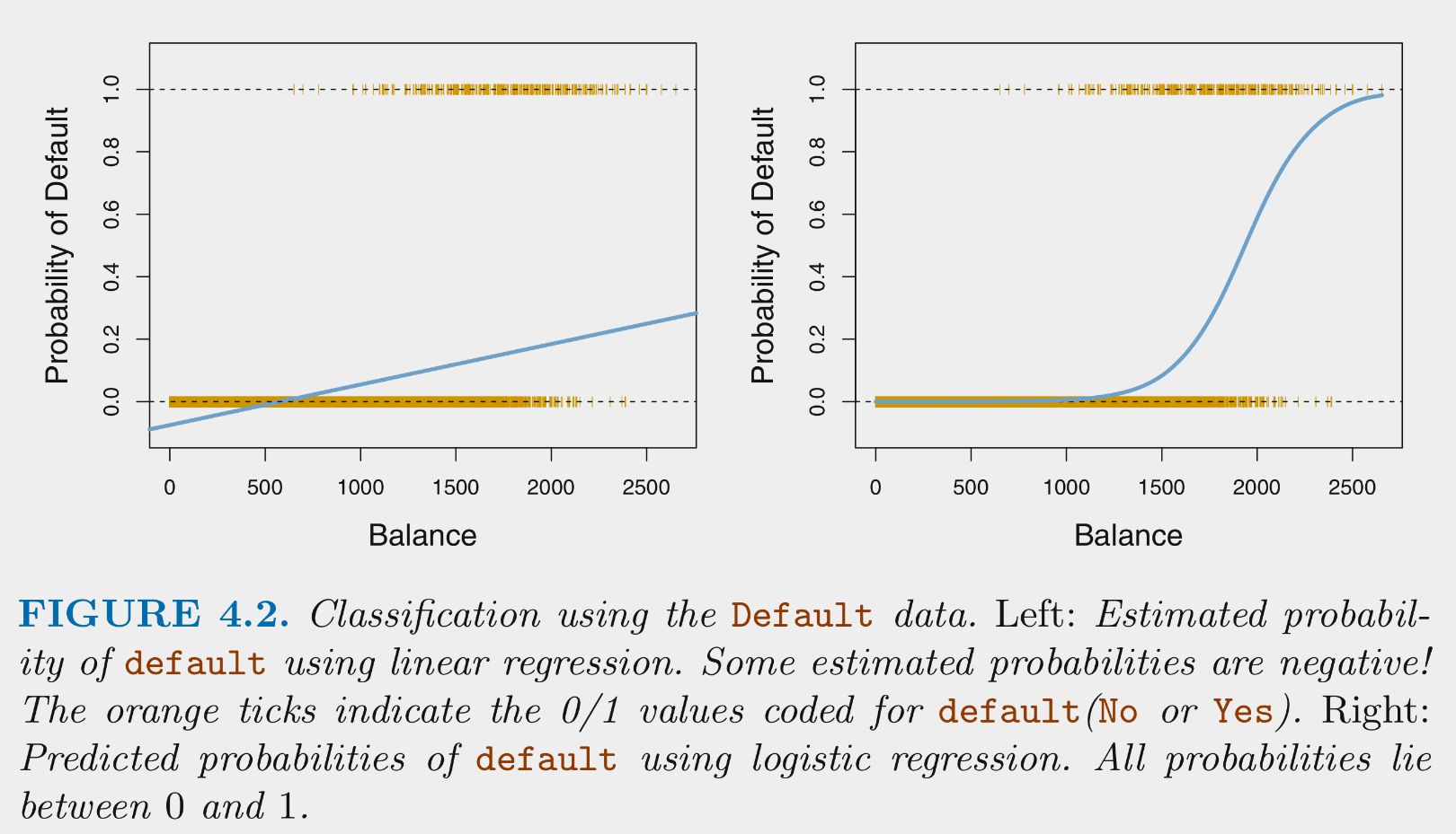
Logistic regression is used frequently for binary and multi-level outcomes because
The general linear model makes predictions that are not bounded by [0, 1] and do not represent true estimates of conditional probability for each class
Logistic regression approaches can be modified to accommodate multi-class outcomes (i.e., more than two levels) even when they are not ordered
Nonetheless, the general linear model is still used at times to predict binary outcomes (see Linear Probability Model) so you should be aware of it. We won’t discuss it further here.
Logistic regression provides predicted conditional probabilities for one class (positive class) for any specific set of values for our features (X)
These conditional probabilities are bounded by [0, 1]
To maximize accuracy (as per Bayes classifier),
we predict the positive case if \(Pr(positive class | X) > .5\) for any specific X
otherwise we predict the negative class
As a simple parametric model, logistic regression is commonly used for explanatory purposes as well as prediction
For these reasons, it is worthwhile to fully understand how to work with the logistic function to quantify and describe the effects of your features/predictors in terms of
Probability
Odds
[Log-odds or logit]
Odds ratio
The logistic function yields the probability of the positive class given X
However, in some instances (e.g., horse racing, poker), it may make more sense to describe the odds of the positive case occurring rather than probability
Odds are defined with respect to probabilities as follows:
As an example, if we fit a logistic regression model to predict the probability of the Badgers winning a home football game given the attendance (measured in individual spectators at the game), we might find \(b_1\) (our estimate of \(\beta_1\)) = .000075.
Given this, the odds ratio associated with every increase in 10,000 spectators:
\(= e^{c * \b_1}\)
\(= e^{10000 * .000075}\)
\(= 2.1\)
For every increase of 10,000 spectators, the odds of the Badgers winning doubles
4.4 The Cars Dataset
Now, let’s put this all of this together in the Cars dataset from Carnegie Mellon’s StatLib Dataset Archive
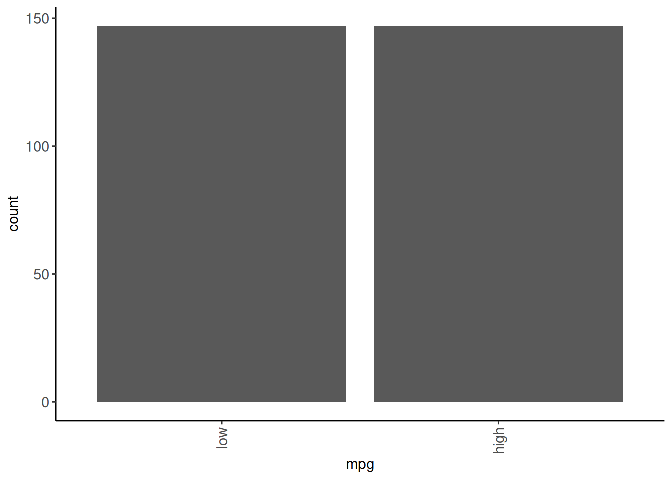
Our goal is to build a classifier (machine learning model for a categorical outcome) that classifies cars as either high or low mpg.
4.4.1 Cleaning EDA
Let’s start with some cleaning EDA
Open and “skim” it RE variable names, classes & missing data
Variable names are already tidy
no missing data
mins (p0) and maxes(p100) for numeric look good
there are two character variables (mpq and name) that will need to be re-classed
mpg is ordinal, so lets set the levels to indicate the order.
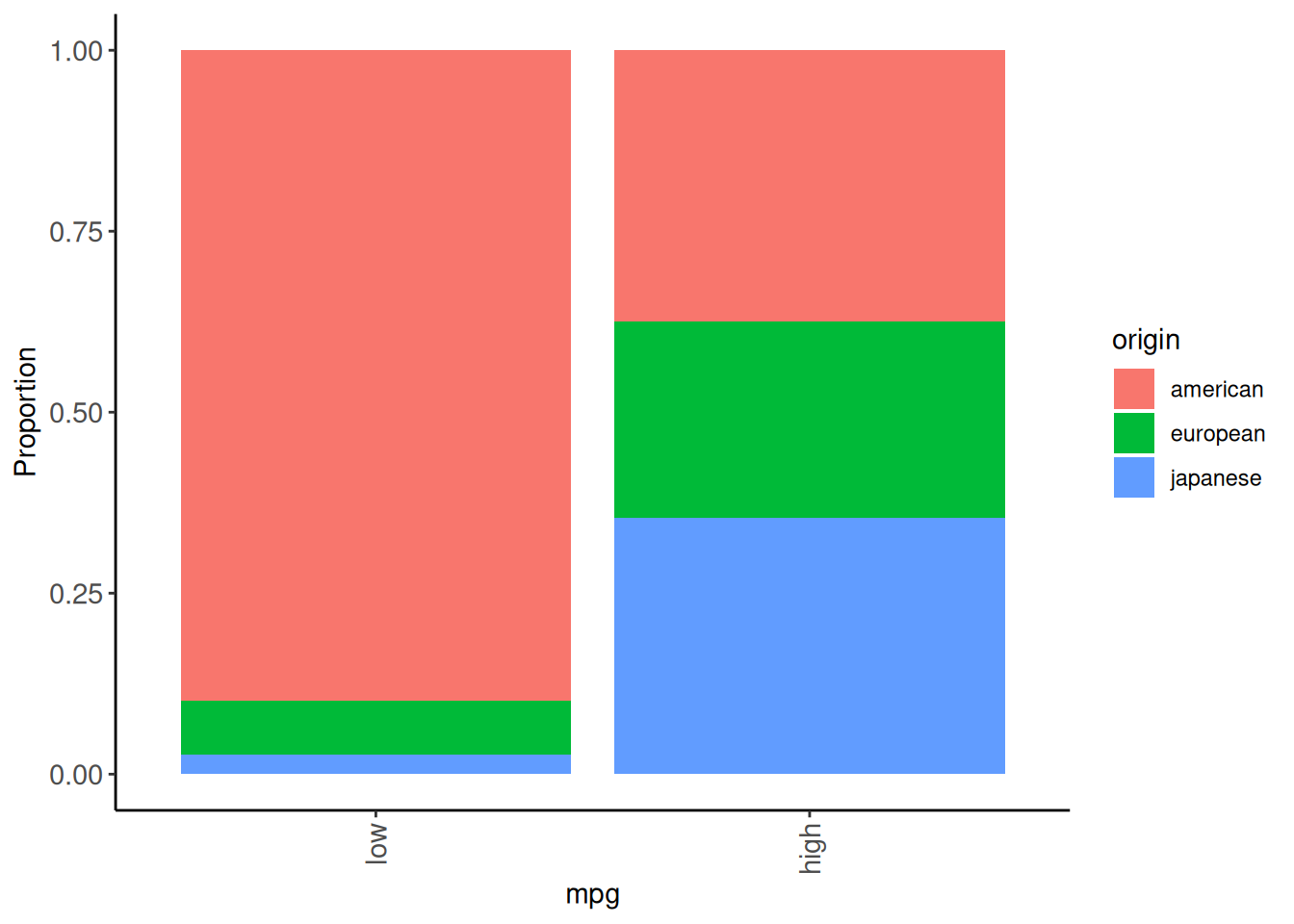
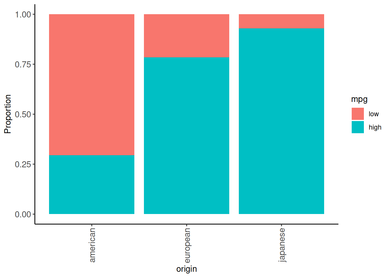
After reviewing the data dictionary, we see that origin is a nominal predictor that is coded numeric (where 1 = American, 2 = European, and 3 = Japanese). Let’s recode as character with meaningful labels and then class as a factor
Finally, let’s make and save our training and validation sets. If we were doing model building for prediction we would also need a test set but we will focus this unit on just selecting the best model but not rigorously evaluating it.
Let’s use a 75/25 split, stratified on mpg
Don’t forget to set a seed in case you need to re-split again in the future!
Any concerns about using this training-validation split?
These sample sizes are starting to get a little small. Fitted models will have higher variance with only 75% (N = 294) observations and performance in validation (with only N = 98 observations) may not be a very precise estimate of true validation error. We will learn more robust methods in the unit on resampling.
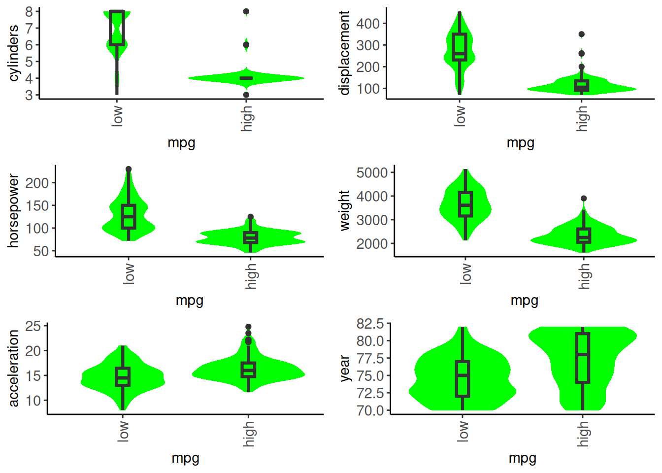
4.4.2 Modeling EDA
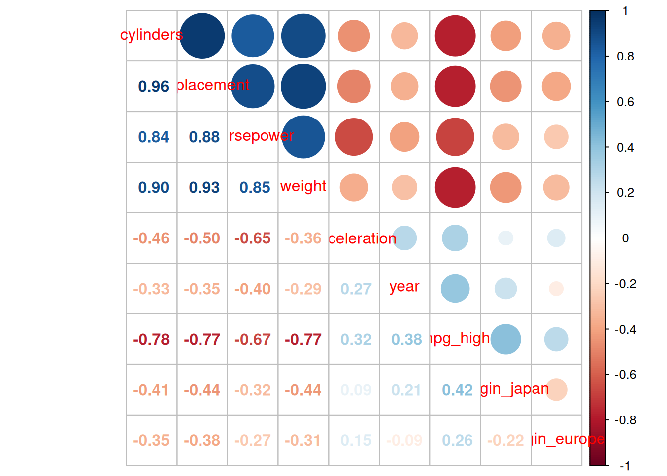
Let’s do some quick modeling EDA to get a sense of the data.
We will keep it quick and dirty.
First, we should make a function to class Cars since we may open it frequently
Even though its simple, still better this way (e.g., what if we decide to change how to handle classing - will only need to make that change in one place!)
If manually coding a binary outcome variable, best practice is to set the positive class to be 1
2
Remove origin and mpg after converting to dummy-coded features
4.5 Logistic Regression - Model Building
Now that we understand our data a little better, let’s build some models
Let’s also try to simultaneously pretend that we:
Are building and selecting a best prediction model that will be evaluated with some additional held out test data (how bad would it have been to split into three sets??!!)
Have an explanatory question about production year - Are we more likely to have efficient cars more recently because of improvements in “technology”, above and beyond broad car characteristics (e.g., the easy stuff like weight, displacement, etc.)
To be clear, prediction and explanation goals are often separate (though prediction is an important foundation explanation)
Set engine to be generalized linear model. No need to `set_mode(“classification”) because logistic regression glm is only used for classification
3
Notice that we explicitly indicate which features to use because our feature matrix has more than just these two in it because we used . in our recipe and our datasets have more columns.
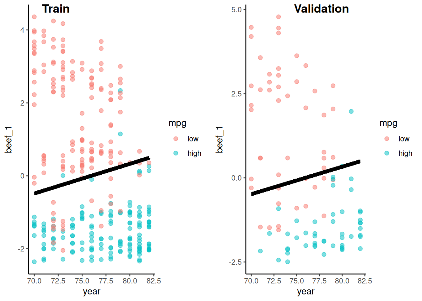
Let’s look at the logistic model and its parameter estimates from train
The preferred test for parameter estimates from logistic regression is the likelihood ratio test
You can get this using Anova() from the car package (as you learn in 610/710)
The glm object is returned using $fit
Code
car::Anova(fit_lr_2$fit, type =3)
Analysis of Deviance Table (Type III tests)

Response: mpg
       LR Chisq Df Pr(>Chisq)
beef_1  239.721  1  < 2.2e-16 ***
year     20.317  1  6.562e-06 ***
---
Signif. codes:  0 '***' 0.001 '**' 0.01 '*' 0.05 '.' 0.1 ' ' 1
Accuracy is a very common performance metric for classification models
How accurate is our two feature model?
Note the use of type = "class"
We can calculate accuracy in the training set. This may be somewhat overfit and optimistic!
Code
accuracy_vec(feat_trn$mpg, predict(fit_lr_2, feat_trn, type ="class")$.pred_class)
[1] 0.9217687
And in the validation set (better estimate of performance in new data. Though if we use this set multiple times to select a best configuration, it will become overfit eventually too!)
Code
accuracy_vec(feat_val$mpg, predict(fit_lr_2, feat_val, type ="class")$.pred_class)
[1] 0.8877551
You can see some evidence of over-fitting to the training set in that model performance is a bit lower in validation
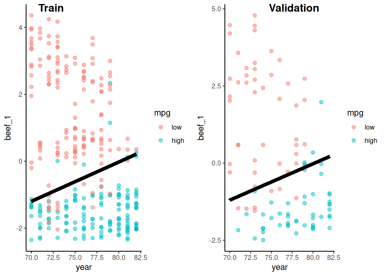
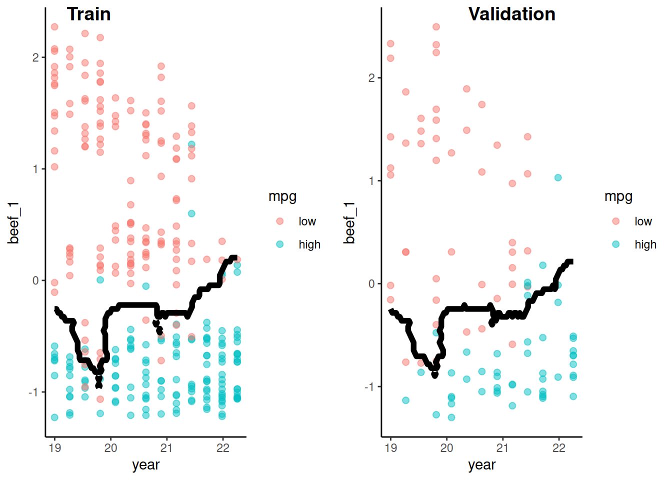
Let’s take a look at the decision boundary for this model in the validation set
We need a function to plot the decision boundary because we will use it repeatedly to compare decision boundaries across statistical models
Displayed here as another example of a function that uses quoted variable names
This function is useful for book examples with two features.
Only can be used with two features, so not that useful in real life!
Not included in my function scripts (just here to help you understand the material)
What if you wanted to try to improve our predictions?
You could find the best set of covariates to test the effect of year. [Assuming the best covariates are those that account for the most variance in mpg]?
For either prediction or explanation, you need to find this best model
We can compare model performance in validation set to find this best model
We can use that one for our prediction goal
We can test the effect of year in that model for our explanation goal
This is a principled way to decide on the best model for our explanatory goal (vs. p-hacking)
We get to explore and we end up with the best model to provide our focal test
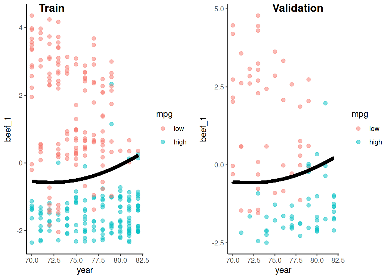
Let’s quickly fit another model we might have considered.
This model will contain the 4 variables from our PCA but as individual features rather than one PCA component score (beef)
Make features for this model
No feature engineering needed because raw variables are all numeric already)
We will give the features dfs new names to retain the old features that included beef_1
The PCA beef model fits best. The model with individual features likely increases overfitting a bit but doesn’t yield a reduction in bias because all the other variables are so highly correlated.
fit_lr_2 is your choice for best model for prediction (at least it is descriptively better)
If you had an explanatory question about year, how would you have chosen between these two tests of year in these two different but all reasonable models
You might have chose the model with individual features because the effect of year is stronger.
That is NOT the model that comes closes to the DGP.
We believe the appropriate model is the beef model that has higher overall accuracy!
This is a start for us to start to consider the use of resampling methods to make decisions about how to best pursue explanatory goals.
Could you now test your year effect in the full sample? Let’s discuss.
Code
car::Anova(fit_lr_2$fit, type =3)
Analysis of Deviance Table (Type III tests)

Response: mpg
       LR Chisq Df Pr(>Chisq)
beef_1  239.721  1  < 2.2e-16 ***
year     20.317  1  6.562e-06 ***
---
Signif. codes:  0 '***' 0.001 '**' 0.01 '*' 0.05 '.' 0.1 ' ' 1
Let’s switch gears to a non-parametric method we already know - KNN.
KNN can be used as a classifier as well as for regression problems
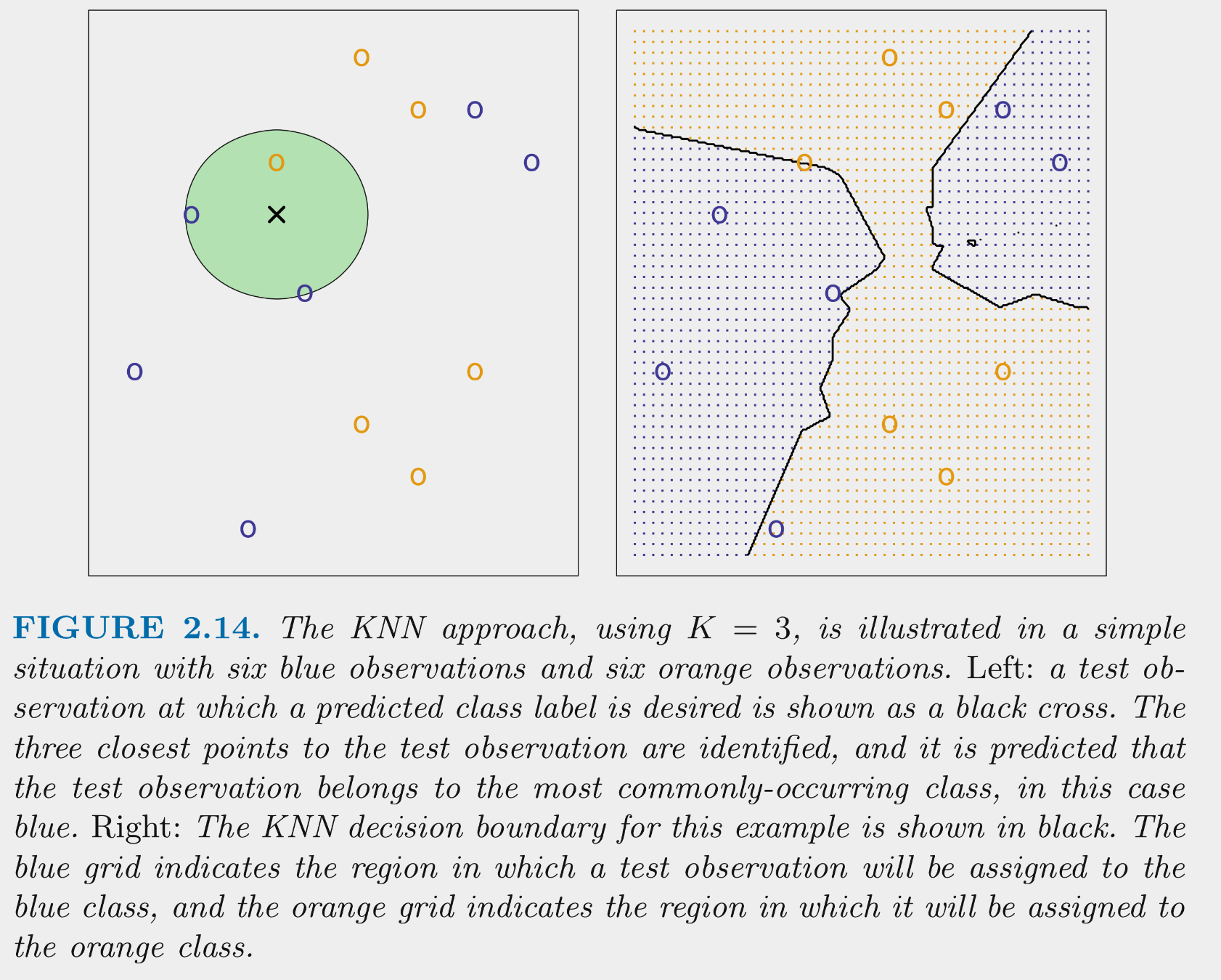
KNN tries to determine conditional class possibilities for any set of features by looking at observed classes for similar values of for these features in the training set
This figure illustrates the application of 3-NN to a small sample training set (N = 12) with 2 predictors
For test observation X in the left panel, we would predict class = blue because blue is the majority class (highest probability) among the 3 nearest training observations
If we calculated these probabilities for all possible combinations of the two predictors in the training set, it would yield the decision boundaries depicted in the right panel
KNN can produce complex decision boundaries
This makes it flexible (can reduce bias)
This makes it susceptible to variance/overfitting problems
Remember that we can control this bias-variance trade-off with K.
As K increases, variance reduces (but bias may increase).
As K decreases, bias may be reduced but variance increases.
Choose a K that produces good performance in new (validation) data
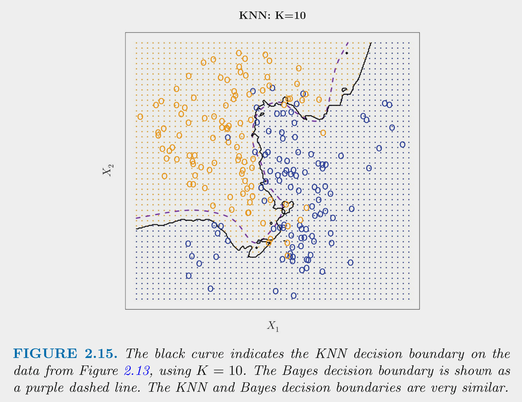
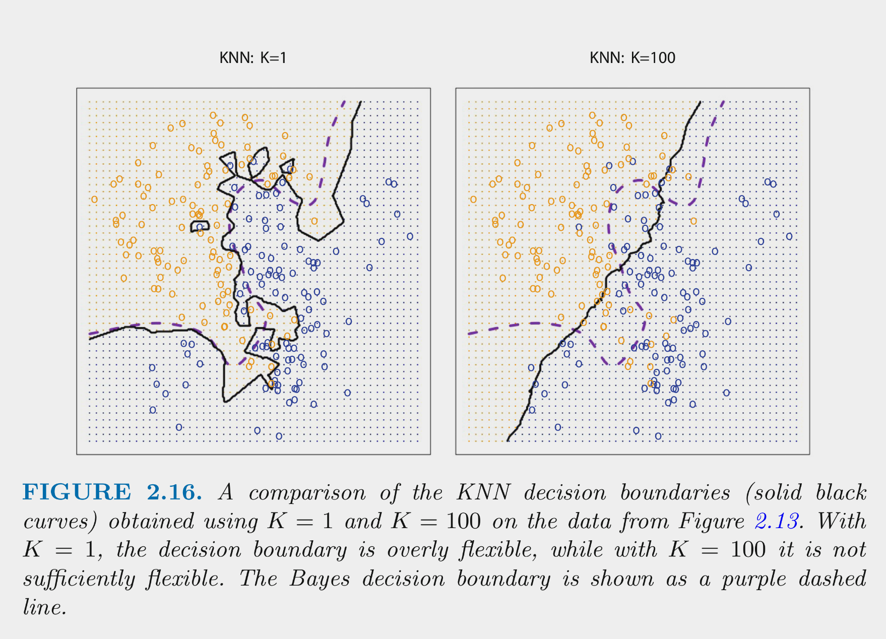
These figures depict the KNN (and Bayes classifier) decision boundaries for the earlier simulated 2 class problem with X1 and X2
K = 10 appears to provide the sweet spot b/c it closely approximates the Bayes decision boundary
Of course, you wouldn’t know the true Bayes decision boundary if the data were real (not simulated)
But K = 10 would also yield the lowest test error (which is how it should be chosen)
Bayes classifier test error: .1304
K = 10 test error: .1363
K = 1 test error: .1695
K = 100 test err: .1925
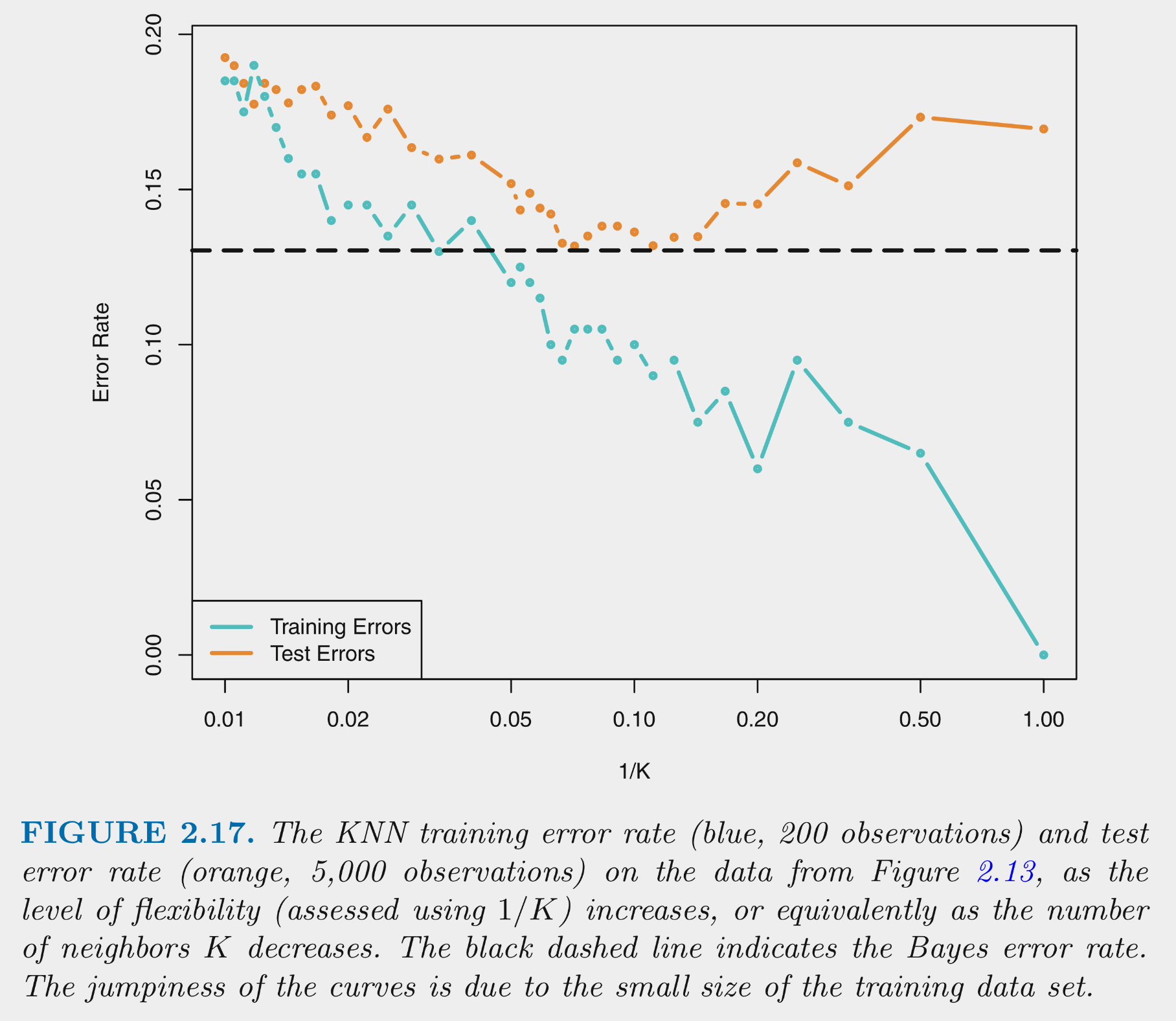
You can NOT make the decision about K based on training error
This figure depicts training and test error for simulated data example as function of 1/K
Training error decreases as 1/K increases. At 1 (K=1) training error is 0
Test error shows expected inverted U
For high K (left side), error is high because of high variance
As move right (lower K), variance is reduced rapidly with little increase in bias. Error is reduced.
Eventually, there is diminishing return from reducing variance but bias starts to increase rapidly. Error increases again.
How do you think the parametric logistic regression compares to the non-parametric KNN with respect to explanatory goals? Consider our (somewhat artificial) question about the effect of year.
The logistic regression provides coefficients (parameter estimates) that can be used to describe changes in probability, odds and odds ratio associated with change in year. These parameter estimates can be tested via inferential procedures.
KNN does not provide any parameter estimates. With KNN, we can visualize decision boundary (only in 2 or three dimensions) or the predicted outcome by any feature, controlling for other features but these relationships may be complex in shape.
Of course, if the relationships are complex, we might not want to hide that.
We will learn more about feature importance for explanation in a later unit.
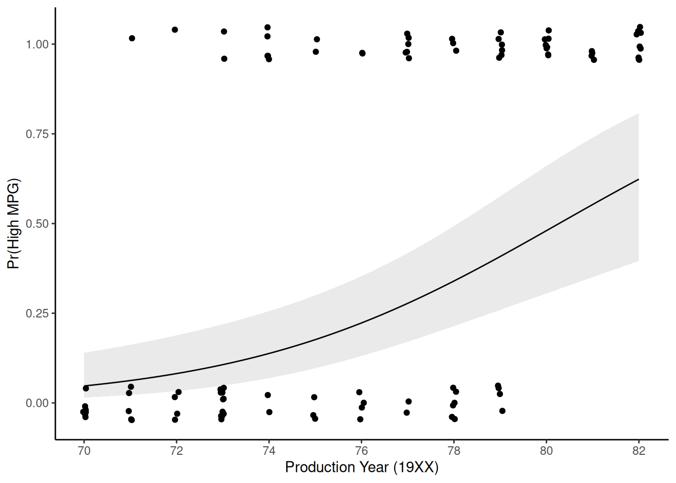
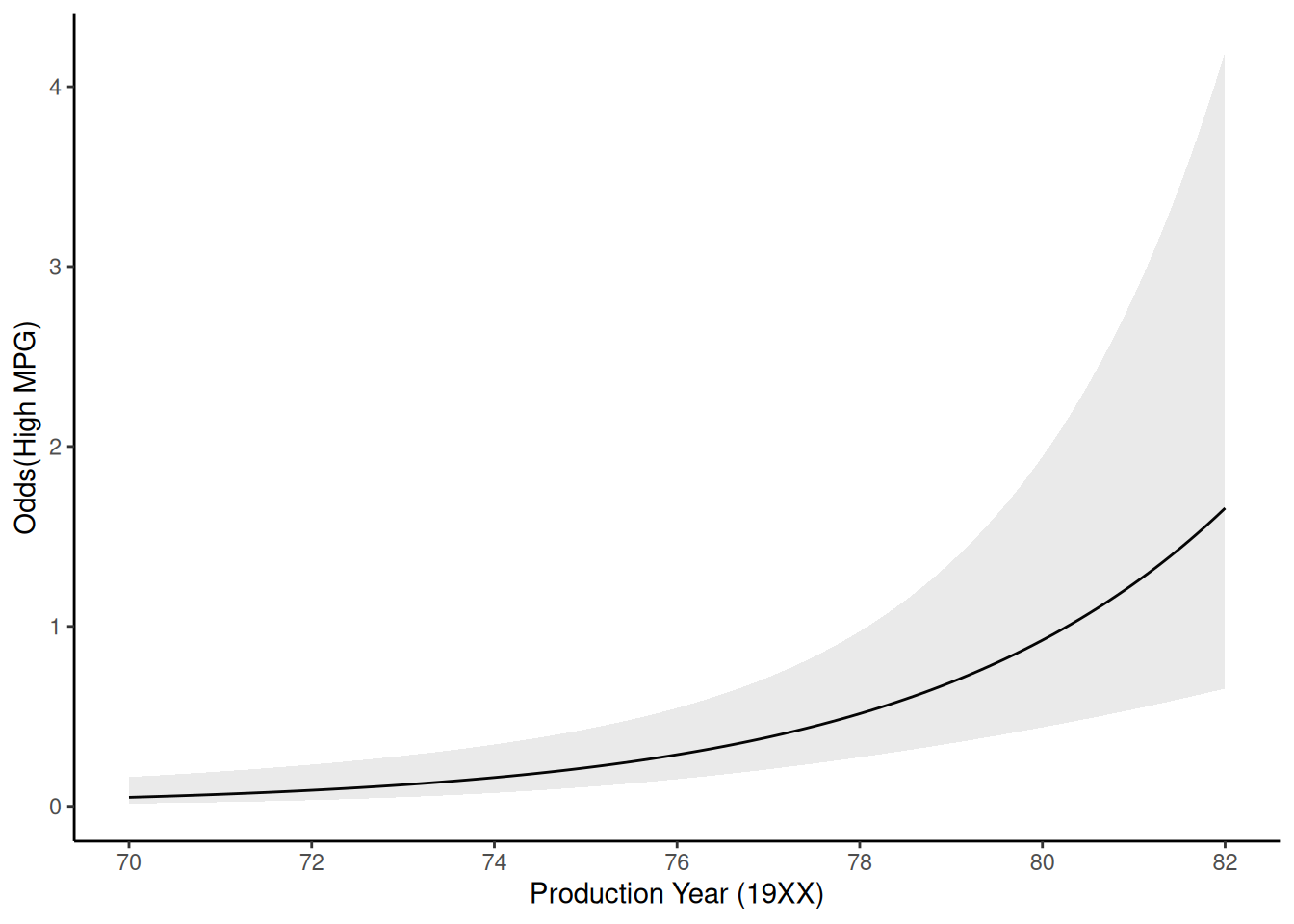
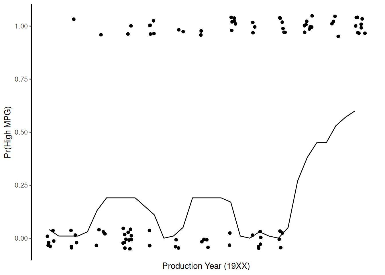
Plot of probability of high_mpg by year, holding beef_1 constant at its mean based on 10-NN
Get \(Pr(high|year)\) holding beef constant at its mean
In a later unit, we will learn about feature ablation that we can combine with model comparisons to potentially test predictor effects in non-parametric models
\(\pi_k\) is the prior probability that an observation comes from class k (estimated from frequencies of k in training)
\(f_k(X)\) is the density function of X for an observation from class k
\(f_k(X)\) is large if there is a high probability that an observation in class k has that set of values for X and small if that probability is low
\(f_k(X)\) is difficult to estimate unless we make some simplifying assumptions (i.e., X is multivariate normal and common covariance matrix (\(\sum\)) across K classes)
With these assumptions, we can estimate \(\pi_k\), \(\mu_k\), and \(\sigma^2\) from the training set and calculate \(Pr(Y = k|X)\) for each k
With a single feature, the probability of any class k, given X is:
LDA is a parametric model, but is it interpretable?
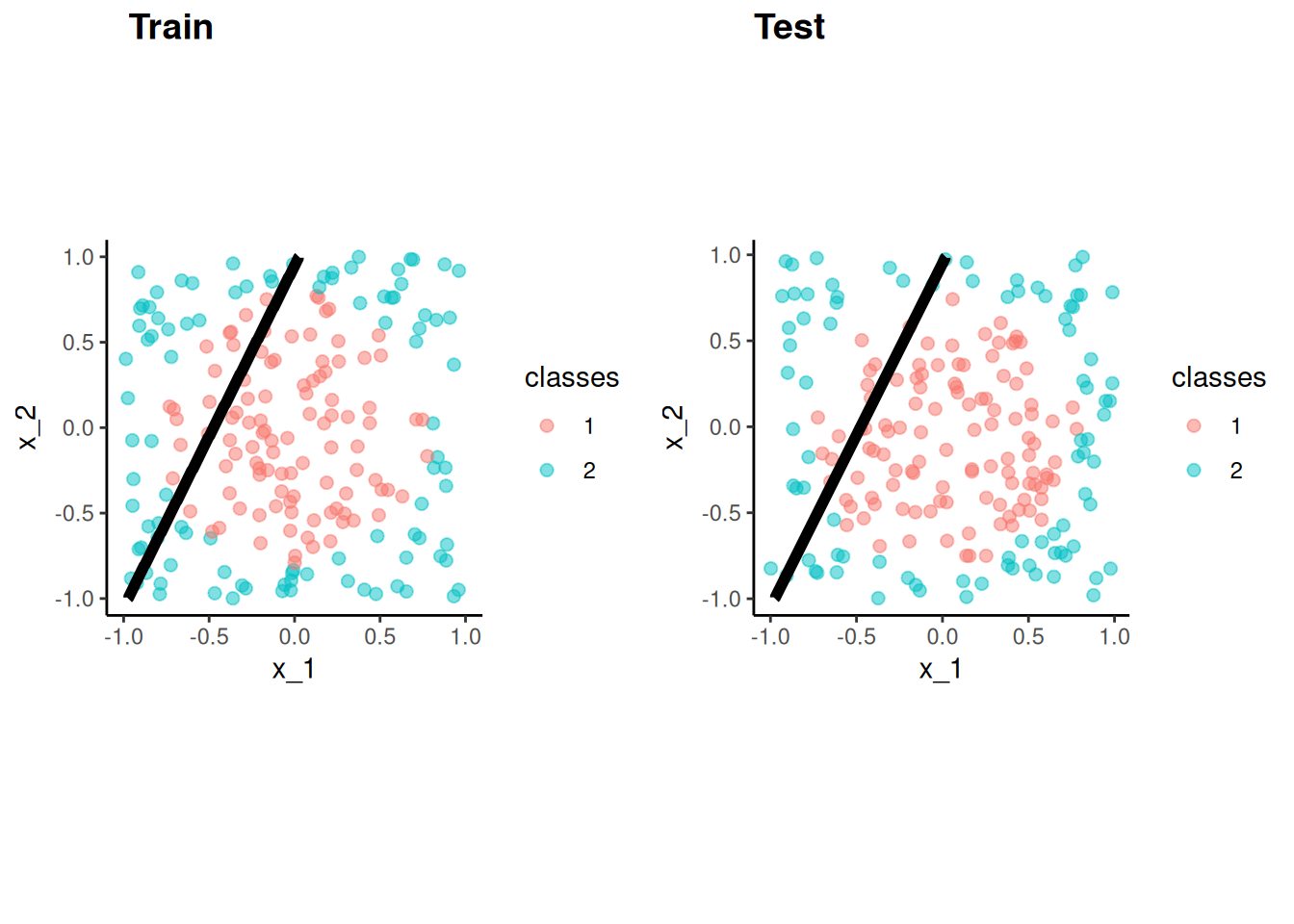
Application of LDA to Cars data set with two predictors
Notice that LDA produces linear decision boundary (see James et al. (2023) for formula for discriminant function derived from the probability function on last slide)
Linear Discriminant Model Specification (classification)

Computational engine: MASS

Model fit template:
MASS::lda(formula = missing_arg(), data = missing_arg())
Both logistic and LDA are linear functions of X and therefore produce linear decision boundaries
LDA makes additional assumptions about X (multivariate normal and common \(\sum\)) beyond logistic regression. Relative performance is based on the quality of this assumption
QDA relaxes the LDA assumption about common \(\sum\) (and RDA can relax it partially)
This also allows for nonlinear decision boundaries including 2-way interactions among features
QDA is therefore more flexible, which means possibly less bias but more potential for overfitting
Both QDA and LDA assume multivariate normal X so may not accommodate categorical predictors very well. Logistic and KNN do accommodate categorical predictors
KNN is non-parametric and therefore the most flexible
Can also handle interactions and non-linear effects natively (with feature engineering)
Increased overfitting, decreased bias?
Not very interpretable. But LDA/QDA, although parametric, aren’t as interpretable as logistic regression
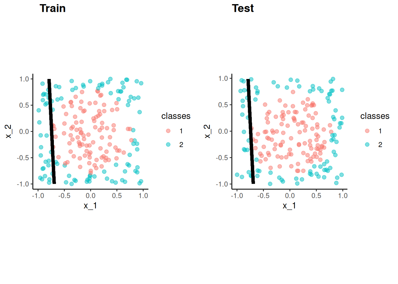
Logistic regression fails when classes are perfectly separated (but does that ever happen?) and is less stable when classes are well separated
LDA, KNN, and QDA naturally accommodate more than two classes
Logistic requires additional tweak (Briefly describe: multiple one vs other classes models approach)
Logistic regression requires relatively large sample sizes. LDA may perform better with smaller sample sizes if assumptions are met. KNN can be computationally very costly with large sample sizes (and large number of X) but could always downsample training set.
4.11 A quick tour of many classifiers
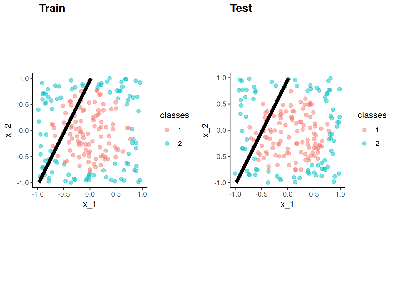
The Cars dataset had strong predictors and a mostly linear decision boundary for the two predictors we considered
This will not be true in many cases
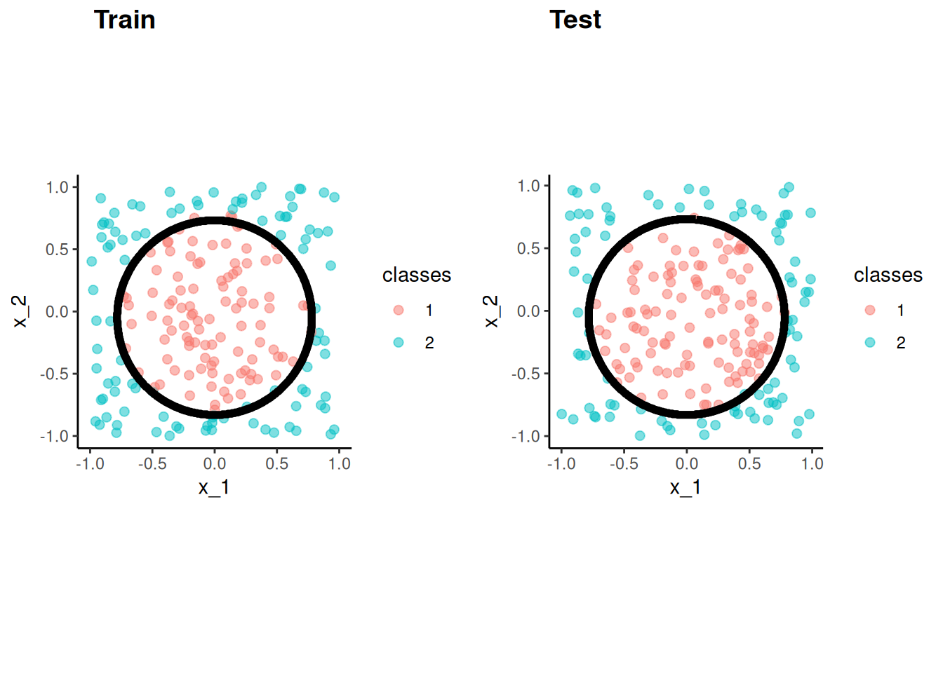
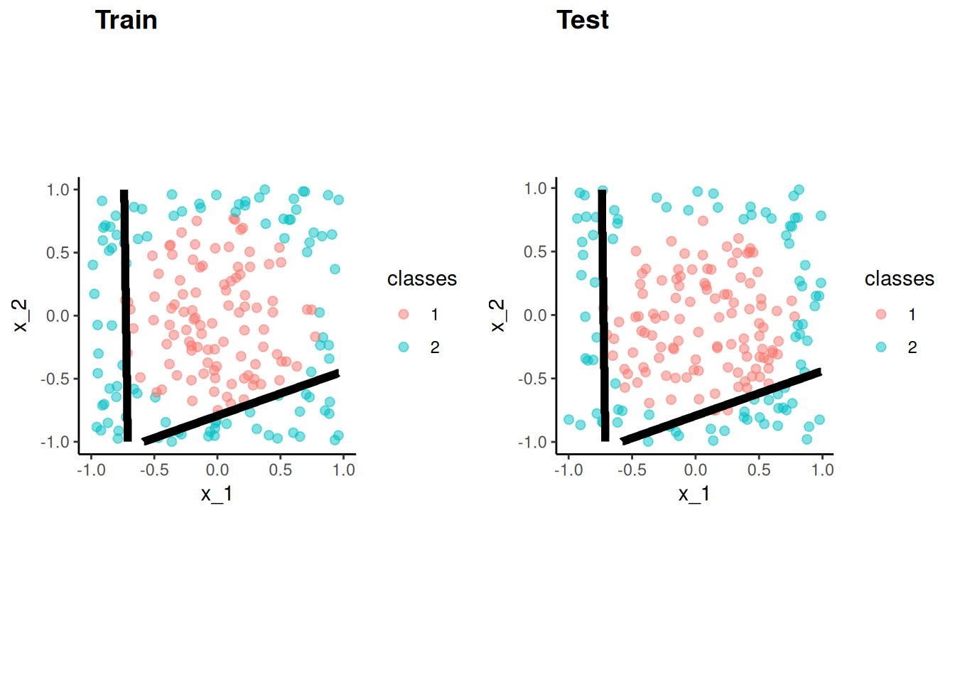
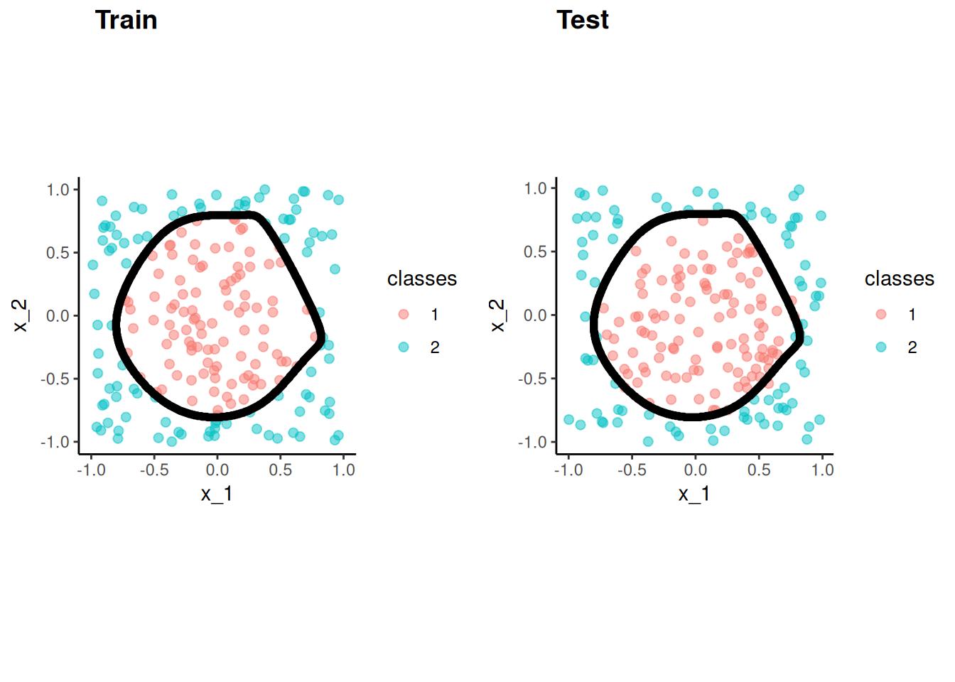
Let’s consider a more complex two predictor decision boundary in the circle dataset from the mlbench package (lots of cool datasets for ML)
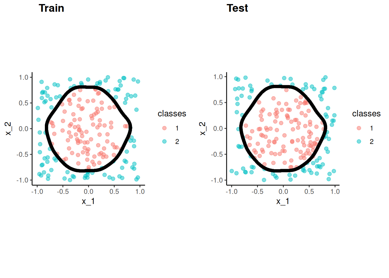
This will hopefully demonstrate that the key is to have a algorithm that can model the DGP
There is NO best algorithm
The best algorithm depends on
The DGP
The goal (prediction vs. explanation)
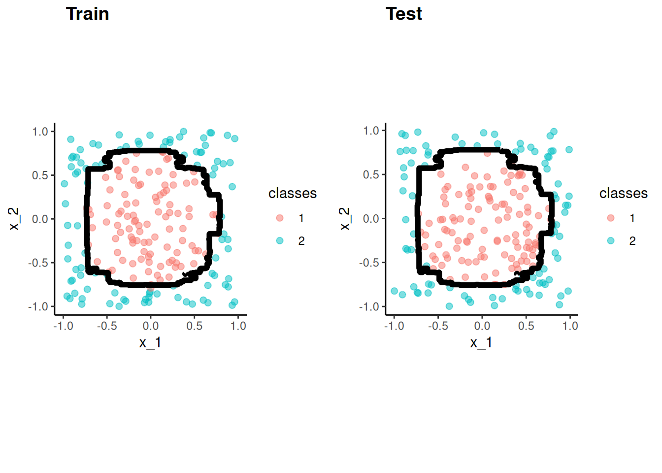
This will also demonstrate the power of tidymodels to allow us to fit many different statistical algorithms which all have their own syntax using a common syntax provided by tidymodels.
This example has been adapted to tidymodels from a demonstration by Michael Hahsler
James, Gareth, Daniela Witten, Trevor Hastie, and Robert Tibshirani. 2023. An Introduction to Statistical Learning: With Applications in R. 2nd ed. Springer Texts in Statistics. Springer-Verlag.