2 Exploratory Data Analysis

2.1 Overview of Unit

2.1.1 Learning Objectives

Stages of Analysis
Best practices for data storage, variable classing, data dictionaries
Problems and solutions regarding data leakage
Key goals and techniques cleaning EDA
- Tidying names and response labels
- Appropriate visualizations based on variable class
- Summary statistics based on variable class
Proper splitting for training/validation and test sets
Key goals and techniques modeling EDA
- Appropriate visualizations based on variable class
- Summary statistics based on variable class
Introductory use of recipes for feature engineering

2.1.2 Readings

[NOTE: These are short chapters. You are reading to understand the framework of visualizing data in R. Don’t feel like you have to memorize the details. These are reference materials that you can turn back to when you need to write code!]

Wickham, Çetinkaya-Rundel, and Grolemund (2023) Chapter 1, Data Visualization
Wickham, Çetinkaya-Rundel, and Grolemund (2023) Chapter 9, Layers
Wickham, Çetinkaya-Rundel, and Grolemund (2023) Chapter 10, Exploratory Data Analysis

Post questions to the readings channel in Slack

2.1.3 Lecture Videos

Lecture 1: Stages of Data Analysis and Model Development ~ 10 mins
Lecture 2: Best Practices and Other Recommendations ~ 27 mins
Lecture 3: EDA for Data Cleaning ~ 41 mins
Lecture 4: EDA for Modeling - Univariate ~ 24 mins
Lecture 5: EDA for Modeling - Bivariate ~ 20 mins
Lecture 6: Working with Recipes ~ 13 mins

Post questions to the video-lectures channel in Slack

2.1.4 Application Assignment and Quiz

data
data dictionary
cleaning EDA: qmd
modeling EDA: qmd
solutions: cleaning EDA; modeling EDA

Post questions to the application-assignments channel in Slack

Submit the application assignment here and complete the unit quiz by 8 pm on Wednesday, January 31st

2.2 Overview of Exploratory Data Analysis

2.2.1 Stages of Data Analysis and Model Development

These are the main stages of data analysis for machine learning and the data that are used

EDA: Cleaning (full dataset)
EDA: Split data into training, validation and test set(s)
EDA: Modeling (training sets)
Model Building: Feature engineering (training sets)
Model Building: Fit many models configurations (training set)
Model Building: Evaluate many models configurations (validation sets)
Final Model Evaluation: Select final/best model configuration (validation sets)
Final Model Evaluation: Fit best model configuration (use both training and validation sets)
Final Model Evaluation: Evaluate final model configuration (test sets)
Final Model Evaluation: Fit best model configuration to ALL data (training, validation, and test sets) if you plan to use it for applications.

The earlier stages are highly iterative:

You may iterate some through EDA stages 1-3 if you find further errors to clean in stage 3 [But make sure you resplit into the same sets]
You will iterate many times though stages 3-6 as you learn more about your data both through EDA for modeling and evaluating actual models in validation

You will NOT iterate back to earlier stages after you select a final model configuration

Stages 7 - 10 are performed ONLY ONCE
Only one model configuration is selected and re-fit and only that model is brought into test for evaluation
Any more than this is essentially equivalent to p-hacking in traditional analyses
Step 10 only happens if you plan to use the model in some application

2.3 Best Practices and Other Recommendations

2.3.1 Data file formats

We generally store data as CSV [comma-separated value] files

Easy to view directly in a text editor
Easy to share because others can use/import into any data analysis platform
Works with version control (e.g. git, svn)
use read_csv() and write_csv()

Exceptions include:

We may consider binary (.rds) format for very big files because read/write can be slow for csv files.
Binary file format provides a very modest additional protection for sensitive data (which we also don’t share)
use read_rds() and write_rds()

See chapter 7 - Data Import in Wickham, Çetinkaya-Rundel, and Grolemund (2023) for more details and advanced techniques for importing data using read_csv()

2.3.2 Classing Variables

We store and class variables in R based on their data type (level of measurement).

See Wikipedia definitions for levels of measurement for a bit more precision that we will provide here.

Coarsely, there are four levels:

nominal: qualitative categories, no inherent order (e.g., marital status, sex, car color)
ordinal: qualitative categories (sometimes uses number), inherent order but not equidistant spacing (e.g., Likert scale; education level)
interval and ratio (generally treated the same in social sciences): quantitative scores, ordered, equidistant spacing. Ratio has true 0. (e.g., temperature in Celsius vs. Kelvin scales)

We generally refer to nominal and ordinal variables as categorical and interval/ratio as quantitative or numeric

For nominal variables

We store (in csv files) these variables as character class with descriptive text labels for the levels
- Easier to share/document
- Reduces errors
We class these variables in R as factors when we load them (using read_csv())
In some cases, we should pay attention to the order of the levels of the variable. e.g.,
- For a dichotomous outcome variable, the positive/event level of dichotomous factor outcome should be first level of the factor
- The order of levels may also matter for factor predictors (e.g., step_dummy() uses first level as reference).

For ordinal variables:

We store (in csv files) these variables as character class with descriptive text labels for the levels
- Easier to share/document
- Reduces errors
We class these variables in R as factors (just like nominal variables)
- It is easier to do EDA with these variables classes as factors
- We use standard factors (not ordered)
Confirm that the order of the levels is set up correctly. This is very important for ordinal variables.
During feature engineering stage, we can then either
- Treat as a nominal variable and create features using step_dummy()
- Treat as an interval variable using step_ordinalscore()

Similar EDA approaches are used with both nominal and ordinal variable

Ordinal variables may show non-linear relations b/c they may not be evenly spaced. In these instances, we can use feature engineering approaches that are also used for nominal variables

For interval and ratio variables:

We store these variables as numeric
We class these variables as numeric (either integer or double - let R decide) during the read and clean stage (They are typically already in this class when read in)

Similar EDA approaches are used with both interval and ratio variables

Similar feature engineering approaches are used with both

2.3.3 Data Dictionaries

You should always make a data dictionary for use with your data files.

Ideally, these are created during the planning phase of your study, prior to the start of data collection
Still useful if created at the start of data analysis

Data dictionaries:

help you keep track of your variables and their characteristics (e.g., valid ranges, valid responses)
can be used by you to check your data during EDA
can be provided to others when you share your data (data are not generally useful to others without a data dictionary)

We will see a variety of data dictionaries throughout the course. Many are not great as you will learn.

2.3.4 The Ames Housing Prices Dataset

We will use the Ames Housing Prices dataset as a running example this unit (and some future units and application assignments as well)

You can read more about the original dataset created by Dean DeCock
The data set contains data from home sales of individual residential property in Ames, Iowa from 2006 to 2010
The original data set includes 2930 observations of sales price and a large number of explanatory variables (23 nominal, 23 ordinal, 14 discrete, and 20 continuous)
This is the original data dictionary
The challenge with this dataset is to build the best possible prediction model for the sale price of the homes.

2.3.5 Packages and Conflicts

First, lets set up our environment with functions from important packages. I strongly recommend reviewing our recommendations for best practices regarding managing function conflicts now. It will save you a lot of headaches in the future.

We set a conflicts policy that will produce errors if we have unanticipated conflicts.
We source a library of functions that we use for common tasks in machine learning.
- This includes a function (tidymodels_conflictRules()) that sets conflict rules to allow us to attach tidymodels functions without conflicts with tidyverse functions.
- You can review that function to see what it does (search for that function name at the link)
Then we use that function

options(conflicts.policy = "depends.ok")
devtools::source_url("https://github.com/jjcurtin/lab_support/blob/main/fun_ml.R?raw=true")
tidymodels_conflictRules()

Next we load packages for functions that we will use regularly. There are five things to note RE best practices

If we will use a lot of functions from a package (e.g., tidyverse, tidymodels), we attach the full package
If we will use only several functions from a package (but plan to use them repeatedly), we use the include.only parameter to just attach those functions.
At times, if we plan to use a single function from a package only 1-2x times, we may not even attach that function at all. Instead, we just call it using its namespace (i.e. packagename::functionname)
If a package has a function that conflicts with our primary packages and we don’t plan to use that function, we load the package but exclude the function. If we really needed it, we can call it with its namespace as per option 3 above.
Pay attention to conflicts that were allowed to make sure you understand and accept them. (I left the package messages and warnings in the book this time to see them. I will hide them to avoid cluttering book in later units but you should always review them.)

1library(janitor, include.only = "clean_names")
2library(cowplot, include.only = "plot_grid")
3library(kableExtra, exclude = "group_rows")
library(tidyverse) 
4library(tidymodels)

1: As an alternative, we could have skipped loading the package and instead called the function as janitor::clean_names()
2: Same is true for cowplot package
3: When loading kableExtra (which we use often), you will always need to exclude groups_rows() to prevent a conflict with dplyr package in the tidyverse
4: Loading tidymodels will produce conflicts unless you source and call my function tidymodels_conflictRules() (see above)

2.3.6 Source and Other Environment Settings

We will also source (from github) two other libraries of functions that we use commonly for exploratory data analyses. You should review these function scripts (fun_eda.R; fun_plots.R to see the code for these functions.

devtools::source_url("https://github.com/jjcurtin/lab_support/blob/main/fun_eda.R?raw=true")
devtools::source_url("https://github.com/jjcurtin/lab_support/blob/main/fun_plots.R?raw=true")

Finally, we tune our environment a bit more by setting plot themes and print options that we prefer

theme_set(theme_classic())
options(tibble.width = Inf, tibble.print_max = Inf)

And we set a relative path to our data. This assumes you are using an RStudio project with the path to the data relative to that project file. I’ve provided more detail elsewhere on best practices for managing files and paths.

path_data <- "data"

2.3.7 Read and Glimpse Dataframe

Lets read in the data and glimpse the subset of observations we will work with in Units 2-3 and the first two application assignments.

1data_all <- read_csv(here::here(path_data, "ames_raw_class.csv"),
2                     col_types = cols()) |>
3  glimpse()

1: First we read data using a relative path and the here::here() function. This is a replacement for file.path() that works better for both interactive use and rendering in Quarto when using projects.
2: We use col_types = cols() to let R guess the correct class for each column. This suppresses messages that aren’t important at this point prior to EDA.
3: It is good practice to always glimpse() data after you read it.

Rows: 1,955
Columns: 81
$ PID               <chr> "0526301100", "0526350040", "0526351010", "052710501…
$ `MS SubClass`     <chr> "020", "020", "020", "060", "120", "120", "120", "06…
$ `MS Zoning`       <chr> "RL", "RH", "RL", "RL", "RL", "RL", "RL", "RL", "RL"…
$ `Lot Frontage`    <dbl> 141, 80, 81, 74, 41, 43, 39, 60, 75, 63, 85, NA, 47,…
$ `Lot Area`        <dbl> 31770, 11622, 14267, 13830, 4920, 5005, 5389, 7500, …
$ Street            <chr> "Pave", "Pave", "Pave", "Pave", "Pave", "Pave", "Pav…
$ Alley             <chr> NA, NA, NA, NA, NA, NA, NA, NA, NA, NA, NA, NA, NA, …
$ `Lot Shape`       <chr> "IR1", "Reg", "IR1", "IR1", "Reg", "IR1", "IR1", "Re…
$ `Land Contour`    <chr> "Lvl", "Lvl", "Lvl", "Lvl", "Lvl", "HLS", "Lvl", "Lv…
$ Utilities         <chr> "AllPub", "AllPub", "AllPub", "AllPub", "AllPub", "A…
$ `Lot Config`      <chr> "Corner", "Inside", "Corner", "Inside", "Inside", "I…
$ `Land Slope`      <chr> "Gtl", "Gtl", "Gtl", "Gtl", "Gtl", "Gtl", "Gtl", "Gt…
$ Neighborhood      <chr> "NAmes", "NAmes", "NAmes", "Gilbert", "StoneBr", "St…
$ `Condition 1`     <chr> "Norm", "Feedr", "Norm", "Norm", "Norm", "Norm", "No…
$ `Condition 2`     <chr> "Norm", "Norm", "Norm", "Norm", "Norm", "Norm", "Nor…
$ `Bldg Type`       <chr> "1Fam", "1Fam", "1Fam", "1Fam", "TwnhsE", "TwnhsE", …
$ `House Style`     <chr> "1Story", "1Story", "1Story", "2Story", "1Story", "1…
$ `Overall Qual`    <dbl> 6, 5, 6, 5, 8, 8, 8, 7, 6, 6, 7, 8, 8, 8, 9, 4, 6, 6…
$ `Overall Cond`    <dbl> 5, 6, 6, 5, 5, 5, 5, 5, 5, 5, 5, 5, 5, 7, 2, 5, 6, 6…
$ `Year Built`      <dbl> 1960, 1961, 1958, 1997, 2001, 1992, 1995, 1999, 1993…
$ `Year Remod/Add`  <dbl> 1960, 1961, 1958, 1998, 2001, 1992, 1996, 1999, 1994…
$ `Roof Style`      <chr> "Hip", "Gable", "Hip", "Gable", "Gable", "Gable", "G…
$ `Roof Matl`       <chr> "CompShg", "CompShg", "CompShg", "CompShg", "CompShg…
$ `Exterior 1st`    <chr> "BrkFace", "VinylSd", "Wd Sdng", "VinylSd", "CemntBd…
$ `Exterior 2nd`    <chr> "Plywood", "VinylSd", "Wd Sdng", "VinylSd", "CmentBd…
$ `Mas Vnr Type`    <chr> "Stone", "None", "BrkFace", "None", "None", "None", …
$ `Mas Vnr Area`    <dbl> 112, 0, 108, 0, 0, 0, 0, 0, 0, 0, 0, 0, 603, 0, 350,…
$ `Exter Qual`      <chr> "TA", "TA", "TA", "TA", "Gd", "Gd", "Gd", "TA", "TA"…
$ `Exter Cond`      <chr> "TA", "TA", "TA", "TA", "TA", "TA", "TA", "TA", "TA"…
$ Foundation        <chr> "CBlock", "CBlock", "CBlock", "PConc", "PConc", "PCo…
$ `Bsmt Qual`       <chr> "TA", "TA", "TA", "Gd", "Gd", "Gd", "Gd", "TA", "Gd"…
$ `Bsmt Cond`       <chr> "Gd", "TA", "TA", "TA", "TA", "TA", "TA", "TA", "TA"…
$ `Bsmt Exposure`   <chr> "Gd", "No", "No", "No", "Mn", "No", "No", "No", "No"…
$ `BsmtFin Type 1`  <chr> "BLQ", "Rec", "ALQ", "GLQ", "GLQ", "ALQ", "GLQ", "Un…
$ `BsmtFin SF 1`    <dbl> 639, 468, 923, 791, 616, 263, 1180, 0, 0, 0, 637, 36…
$ `BsmtFin Type 2`  <chr> "Unf", "LwQ", "Unf", "Unf", "Unf", "Unf", "Unf", "Un…
$ `BsmtFin SF 2`    <dbl> 0, 144, 0, 0, 0, 0, 0, 0, 0, 0, 0, 1120, 0, 0, 0, 0,…
$ `Bsmt Unf SF`     <dbl> 441, 270, 406, 137, 722, 1017, 415, 994, 763, 789, 6…
$ `Total Bsmt SF`   <dbl> 1080, 882, 1329, 928, 1338, 1280, 1595, 994, 763, 78…
$ Heating           <chr> "GasA", "GasA", "GasA", "GasA", "GasA", "GasA", "Gas…
$ `Heating QC`      <chr> "Fa", "TA", "TA", "Gd", "Ex", "Ex", "Ex", "Gd", "Gd"…
$ `Central Air`     <chr> "Y", "Y", "Y", "Y", "Y", "Y", "Y", "Y", "Y", "Y", "Y…
$ Electrical        <chr> "SBrkr", "SBrkr", "SBrkr", "SBrkr", "SBrkr", "SBrkr"…
$ `1st Flr SF`      <dbl> 1656, 896, 1329, 928, 1338, 1280, 1616, 1028, 763, 7…
$ `2nd Flr SF`      <dbl> 0, 0, 0, 701, 0, 0, 0, 776, 892, 676, 0, 0, 1589, 67…
$ `Low Qual Fin SF` <dbl> 0, 0, 0, 0, 0, 0, 0, 0, 0, 0, 0, 0, 0, 0, 0, 0, 0, 0…
$ `Gr Liv Area`     <dbl> 1656, 896, 1329, 1629, 1338, 1280, 1616, 1804, 1655,…
$ `Bsmt Full Bath`  <dbl> 1, 0, 0, 0, 1, 0, 1, 0, 0, 0, 1, 1, 1, 0, 1, 0, 1, 0…
$ `Bsmt Half Bath`  <dbl> 0, 0, 0, 0, 0, 0, 0, 0, 0, 0, 0, 0, 0, 0, 0, 0, 0, 0…
$ `Full Bath`       <dbl> 1, 1, 1, 2, 2, 2, 2, 2, 2, 2, 1, 1, 3, 2, 1, 1, 2, 2…
$ `Half Bath`       <dbl> 0, 0, 1, 1, 0, 0, 0, 1, 1, 1, 1, 1, 1, 0, 1, 0, 0, 0…
$ `Bedroom AbvGr`   <dbl> 3, 2, 3, 3, 2, 2, 2, 3, 3, 3, 2, 1, 4, 4, 1, 2, 3, 3…
$ `Kitchen AbvGr`   <dbl> 1, 1, 1, 1, 1, 1, 1, 1, 1, 1, 1, 1, 1, 1, 1, 1, 1, 1…
$ `Kitchen Qual`    <chr> "TA", "TA", "Gd", "TA", "Gd", "Gd", "Gd", "Gd", "TA"…
$ `TotRms AbvGrd`   <dbl> 7, 5, 6, 6, 6, 5, 5, 7, 7, 7, 5, 4, 12, 8, 8, 4, 7, …
$ Functional        <chr> "Typ", "Typ", "Typ", "Typ", "Typ", "Typ", "Typ", "Ty…
$ Fireplaces        <dbl> 2, 0, 0, 1, 0, 0, 1, 1, 1, 1, 1, 0, 1, 0, 1, 0, 2, 1…
$ `Fireplace Qu`    <chr> "Gd", NA, NA, "TA", NA, NA, "TA", "TA", "TA", "Gd", …
$ `Garage Type`     <chr> "Attchd", "Attchd", "Attchd", "Attchd", "Attchd", "A…
$ `Garage Yr Blt`   <dbl> 1960, 1961, 1958, 1997, 2001, 1992, 1995, 1999, 1993…
$ `Garage Finish`   <chr> "Fin", "Unf", "Unf", "Fin", "Fin", "RFn", "RFn", "Fi…
$ `Garage Cars`     <dbl> 2, 1, 1, 2, 2, 2, 2, 2, 2, 2, 2, 2, 3, 2, 3, 2, 2, 2…
$ `Garage Area`     <dbl> 528, 730, 312, 482, 582, 506, 608, 442, 440, 393, 50…
$ `Garage Qual`     <chr> "TA", "TA", "TA", "TA", "TA", "TA", "TA", "TA", "TA"…
$ `Garage Cond`     <chr> "TA", "TA", "TA", "TA", "TA", "TA", "TA", "TA", "TA"…
$ `Paved Drive`     <chr> "P", "Y", "Y", "Y", "Y", "Y", "Y", "Y", "Y", "Y", "Y…
$ `Wood Deck SF`    <dbl> 210, 140, 393, 212, 0, 0, 237, 140, 157, 0, 192, 0, …
$ `Open Porch SF`   <dbl> 62, 0, 36, 34, 0, 82, 152, 60, 84, 75, 0, 54, 36, 12…
$ `Enclosed Porch`  <dbl> 0, 0, 0, 0, 170, 0, 0, 0, 0, 0, 0, 0, 0, 0, 0, 0, 0,…
$ `3Ssn Porch`      <dbl> 0, 0, 0, 0, 0, 0, 0, 0, 0, 0, 0, 0, 0, 0, 0, 0, 0, 0…
$ `Screen Porch`    <dbl> 0, 120, 0, 0, 0, 144, 0, 0, 0, 0, 0, 140, 210, 0, 0,…
$ `Pool Area`       <dbl> 0, 0, 0, 0, 0, 0, 0, 0, 0, 0, 0, 0, 0, 0, 0, 0, 0, 0…
$ `Pool QC`         <chr> NA, NA, NA, NA, NA, NA, NA, NA, NA, NA, NA, NA, NA, …
$ Fence             <chr> NA, "MnPrv", NA, "MnPrv", NA, NA, NA, NA, NA, NA, NA…
$ `Misc Feature`    <chr> NA, NA, "Gar2", NA, NA, NA, NA, NA, NA, NA, NA, NA, …
$ `Misc Val`        <dbl> 0, 0, 12500, 0, 0, 0, 0, 0, 0, 0, 0, 0, 0, 0, 0, 0, …
$ `Mo Sold`         <dbl> 5, 6, 6, 3, 4, 1, 3, 6, 4, 5, 2, 6, 6, 6, 6, 6, 2, 1…
$ `Yr Sold`         <dbl> 2010, 2010, 2010, 2010, 2010, 2010, 2010, 2010, 2010…
$ `Sale Type`       <chr> "WD", "WD", "WD", "WD", "WD", "WD", "WD", "WD", "WD"…
$ `Sale Condition`  <chr> "Normal", "Normal", "Normal", "Normal", "Normal", "N…
$ SalePrice         <dbl> 215000, 105000, 172000, 189900, 213500, 191500, 2365…

Dataset Notes:

Dataset has N = 1955 rather than 2930.
- I have held out remaining observations to serve as a test set for a friendly competition in Unit 3
- I will judge your models’ performance with this test set at that time!
- More on the importance of held out test sets as we progress through the course
This full dataset has 81 variables. For the lecture examples in units 2-3 we will only use a subset of the predictors
You will use different predictors in the next two application assignments

Here we select the variables we will use for lecture

data_all <- data_all |> 
  select(SalePrice,
         `Gr Liv Area`, 
         `Lot Area`, 
         `Year Built`, 
         `Overall Qual`, 
         `Garage Cars`,
         `Garage Qual`,
         `MS Zoning`,
         `Lot Config` ,
1         `Bldg Type`) |>
  glimpse()

1: Notice that the dataset used non-standard variable names that include spaces. We need to use back-ticks around the variable names to allow us reference those variables. We will fix this during the cleaning process and you should never use spaces in variable names when setting up your own data!!!

Rows: 1,955
Columns: 10
$ SalePrice      <dbl> 215000, 105000, 172000, 189900, 213500, 191500, 236500,…
$ `Gr Liv Area`  <dbl> 1656, 896, 1329, 1629, 1338, 1280, 1616, 1804, 1655, 14…
$ `Lot Area`     <dbl> 31770, 11622, 14267, 13830, 4920, 5005, 5389, 7500, 100…
$ `Year Built`   <dbl> 1960, 1961, 1958, 1997, 2001, 1992, 1995, 1999, 1993, 1…
$ `Overall Qual` <dbl> 6, 5, 6, 5, 8, 8, 8, 7, 6, 6, 7, 8, 8, 8, 9, 4, 6, 6, 7…
$ `Garage Cars`  <dbl> 2, 1, 1, 2, 2, 2, 2, 2, 2, 2, 2, 2, 3, 2, 3, 2, 2, 2, 2…
$ `Garage Qual`  <chr> "TA", "TA", "TA", "TA", "TA", "TA", "TA", "TA", "TA", "…
$ `MS Zoning`    <chr> "RL", "RH", "RL", "RL", "RL", "RL", "RL", "RL", "RL", "…
$ `Lot Config`   <chr> "Corner", "Inside", "Corner", "Inside", "Inside", "Insi…
$ `Bldg Type`    <chr> "1Fam", "1Fam", "1Fam", "1Fam", "TwnhsE", "TwnhsE", "Tw…

2.4 Exploratory Data Analysis for Data Cleaning

EDA could be done using either tidyverse packages and functions or tidymodels (mostly using the recipes package.)

We prefer to use the richer set of functions available in the tidyverse (and dplyr and purrr packages in particular).
We will reserve the use of recipes for feature engineering only when we are building features for models that we will fit in our training sets and evaluation in our validation and test sets.

2.4.1 Data Leakage Issues

Data leakage refers to a mistake made by the developer of a machine learning model in which they accidentally share information between their training set and held-out validation or test sets

Training sets are used to fit models with different configurations
Validation sets are used to select the best model among those with different configurations (not needed if you only have one configuration)
Test sets are used to evaluate a best model
When splitting data-sets into training, validation and test sets, the goal is to ensure that no data (or information more broadly) are shared between the three sets
- No data or information from test should influence either fitting or selecting models
- Test should only be used once to evaluate a best/final model
- Train and validation set also must be segregated (although validation sets may be used to evaluate many model configurations)
- Information necessary for transformations and other feature engineering (e.g., means/sds for centering/scaling, procedures for missing data imputation) must all be based only on training data.
- Data leakage is common if you are not careful.

In particular, if we begin to use test data or information about test during model fitting

We risk overfitting
This is essentially the equivalent of p-hacking in traditional analyses
Our estimate of model performance will be too optimistic, which could have harmful real-world consequences.

2.4.2 Tidy variable names

Use snake case for variable names

clean_names() from janitor package is useful for this.
May need to do further correction of variable names using rename()
See more details about tidy names for objects (e.g., variables, dfs, functions) per Tidy Style Guide

data_all <- data_all |> 
  clean_names("snake")

data_all |> names()

 [1] "sale_price"   "gr_liv_area"  "lot_area"     "year_built"   "overall_qual"
 [6] "garage_cars"  "garage_qual"  "ms_zoning"    "lot_config"   "bldg_type"

2.4.3 Explore variable classes

At this point, we should class all of our variables as either numeric or factor

Interval and ratio variables use numeric classes (dbl or int)
Nominal and ordinal variable use factor class
Useful for variable selection later (e.g., where(is.numeric), where(is.factor))

Subsequent cleaning steps are clearer if we have this established/confirmed now

We have a number of nominal or ordinal variables that are classed as character.

We have one ordinal variable (overall_qual) that is classed as numeric (because the levels were coded with numbers rather than text)

read_csv() thought was numeric by the levels are coded using numbers
The data dictionary indicates that valid values range from 1 - 10.

data_all |> glimpse()

Rows: 1,955
Columns: 10
$ sale_price   <dbl> 215000, 105000, 172000, 189900, 213500, 191500, 236500, 1…
$ gr_liv_area  <dbl> 1656, 896, 1329, 1629, 1338, 1280, 1616, 1804, 1655, 1465…
$ lot_area     <dbl> 31770, 11622, 14267, 13830, 4920, 5005, 5389, 7500, 10000…
$ year_built   <dbl> 1960, 1961, 1958, 1997, 2001, 1992, 1995, 1999, 1993, 199…
$ overall_qual <dbl> 6, 5, 6, 5, 8, 8, 8, 7, 6, 6, 7, 8, 8, 8, 9, 4, 6, 6, 7, …
$ garage_cars  <dbl> 2, 1, 1, 2, 2, 2, 2, 2, 2, 2, 2, 2, 3, 2, 3, 2, 2, 2, 2, …
$ garage_qual  <chr> "TA", "TA", "TA", "TA", "TA", "TA", "TA", "TA", "TA", "TA…
$ ms_zoning    <chr> "RL", "RH", "RL", "RL", "RL", "RL", "RL", "RL", "RL", "RL…
$ lot_config   <chr> "Corner", "Inside", "Corner", "Inside", "Inside", "Inside…
$ bldg_type    <chr> "1Fam", "1Fam", "1Fam", "1Fam", "TwnhsE", "TwnhsE", "Twnh…

We can the recode overall_qual first and set its levels

We can recode all the character variables to factor in one step. Most are nominal. We will handle the order for garage_qual later.

1oq_levels <- 1:10

data_all <-  data_all |> 
  mutate(overall_qual = factor(overall_qual, 
2                               levels = oq_levels)) |>
3  mutate(across(where(is.character), factor)) |>
  glimpse()

1: It is always best to explicitly set the levels of an ordinal factor in the order you prefer. It is not necessary here because overall_qual was numeric and therefore sorts in the expected order. However, if it had been numbers stored as characters, it could sort incorrectly (e.g., 1, 10, 2, 3, …). And obviously if the orders levels were names, the order would have to be specified.
2: We indicate the levels here.
3: We use a mutate to re-class all character data to factors. I prefer factor() to forcats::fct() because factor orders the levels alphabetically. Be aware that this could change if your code is used in a region of the world where this sorting is different. I still prefer this to the alternative (in fct()) that orders by the order the levels are found in your data.

Rows: 1,955
Columns: 10
$ sale_price   <dbl> 215000, 105000, 172000, 189900, 213500, 191500, 236500, 1…
$ gr_liv_area  <dbl> 1656, 896, 1329, 1629, 1338, 1280, 1616, 1804, 1655, 1465…
$ lot_area     <dbl> 31770, 11622, 14267, 13830, 4920, 5005, 5389, 7500, 10000…
$ year_built   <dbl> 1960, 1961, 1958, 1997, 2001, 1992, 1995, 1999, 1993, 199…
$ overall_qual <fct> 6, 5, 6, 5, 8, 8, 8, 7, 6, 6, 7, 8, 8, 8, 9, 4, 6, 6, 7, …
$ garage_cars  <dbl> 2, 1, 1, 2, 2, 2, 2, 2, 2, 2, 2, 2, 3, 2, 3, 2, 2, 2, 2, …
$ garage_qual  <fct> TA, TA, TA, TA, TA, TA, TA, TA, TA, TA, TA, TA, TA, TA, T…
$ ms_zoning    <fct> RL, RH, RL, RL, RL, RL, RL, RL, RL, RL, RL, RL, RL, RL, R…
$ lot_config   <fct> Corner, Inside, Corner, Inside, Inside, Inside, Inside, I…
$ bldg_type    <fct> 1Fam, 1Fam, 1Fam, 1Fam, TwnhsE, TwnhsE, TwnhsE, 1Fam, 1Fa…

2.4.4 Skimming the data

skim() from the skimr package is a wonderful and customizable function for summary statistics

It is highly customizable so we can write our own versions for our own needs
We use different versions for cleaning and modeling EDA
For cleaning EDA, we just remove some stats that we don’t want to see at this time
We can get many of the summary stats for cleaning in one call
We have a custom skim defined in the fun_eda.R function library that we use regularly. Here is the code but you can use the function directly if you sourced fun_eda.R (as we did above)

skim_some <- skim_with(numeric = sfl(mean = NULL, sd = NULL, p25 = NULL, p50 = NULL, p75 = NULL, hist = NULL))

Here is what we get with our new skim_some() function

We will refer to this again for each characteristic we want to review for instructional purposes
We can already see that we can use skim_some() to confirm that we only have numeric and factor classes

data_all |> 
  skim_some()

Data summary
Name	data_all
Number of rows	1955
Number of columns	10
_______________________
Column type frequency:
factor	5
numeric	5
________________________
Group variables	None

Variable type: factor

skim_variable	n_missing	complete_rate	ordered	n_unique	top_counts
overall_qual	0	1.00	FALSE	10	5: 556, 6: 487, 7: 403, 8: 233
garage_qual	109	0.94	FALSE	5	TA: 1745, Fa: 79, Gd: 16, Po: 4
ms_zoning	0	1.00	FALSE	7	RL: 1530, RM: 297, FV: 91, C (: 19
lot_config	0	1.00	FALSE	5	Ins: 1454, Cor: 328, Cul: 114, FR2: 55
bldg_type	0	1.00	FALSE	5	1Fa: 1631, Twn: 145, Dup: 77, Twn: 64

Variable type: numeric

skim_variable	n_missing	complete_rate	p0	p100
sale_price	0	1	12789	745000
gr_liv_area	0	1	438	5642
lot_area	0	1	1476	215245
year_built	0	1	1875	2010
garage_cars	1	1	0	4

Coding sidebar 1:

Write functions whenever you will repeat code often. You can now reuse skim_some()
skim_with() is an example of a function factory - a function that is used to create a new function
- partial() and compose() are two other function factories we will use at times
- More details on function factories is available in Advanced R

Coding sidebar 2:

Gather useful functions together in a script that you can reuse.
All of the reusable functions in this and later units are available to you in one of my public github repositories.
You can load these functions into your workspace directly from github using devtools::source_url(). For example: devtools::source_url("https://github.com/jjcurtin/lab_support/blob/main/fun_modeling.R?raw=true")
You should start to gather your favorite custom functions together in your own script(s).
You can save your own scripts in a local file and load them into your workspace using source() or you can make your own github repo so you can begin to share your code with others!

2.4.5 Missing Data - All variables

skim_some() provides us with missing data counts and complete data proportions for each variable

data_all |> 
  skim_some() |> 
1  select(skim_variable, n_missing, complete_rate)

1: skim_some() returns a dataframe so you can select only the subset of columns to focus its output on what you want. Or just print it all!

# A tibble: 10 × 3
   skim_variable n_missing complete_rate
   <chr>             <int>         <dbl>
 1 overall_qual          0         1    
 2 garage_qual         109         0.944
 3 ms_zoning             0         1    
 4 lot_config            0         1    
 5 bldg_type             0         1    
 6 sale_price            0         1    
 7 gr_liv_area           0         1    
 8 lot_area              0         1    
 9 year_built            0         1    
10 garage_cars           1         0.999

You likely should view the full observation for missing values

We will show you a few methods to do this in your rendered output

print() will print only 20 rows and the number of columns that will display for width of page
- Set options() if you will do a lot of printing and want full dataframe printed
Use kbl() from kableExtra package for formatted tables (two methods below)

Don’t forget that you can also use View() interactively in R Studio

Option 1 (Simple): Use print() with options()

1options(tibble.width = Inf, tibble.print_max = Inf)

data_all |> filter(is.na(garage_cars)) |> 
  print()

1: This sets print to print all rows and columns. Note that we set these options at the start of the unit b.c. we like to see our full tibbles. If we want only a subset of the first (or last) rows, we use head() or tail()

# A tibble: 1 × 10
  sale_price gr_liv_area lot_area year_built overall_qual garage_cars
       <dbl>       <dbl>    <dbl>      <dbl> <fct>              <dbl>
1     150909        1828     9060       1923 5                     NA
  garage_qual ms_zoning lot_config bldg_type
  <fct>       <fct>     <fct>      <fct>    
1 <NA>        RM        Inside     1Fam

Here are some more advanced options using kbl() for the df with many rows

kable() tables from knitr package and kableExtra extensions (including kbl()) are very useful during EDA and also final publication quality tables
use library(kableExtra)
see vignettes for kableExtra

Option 2 (more advanced): Use a function for kables that we created. Code is displayed here but the function is available to you if you source fun_eda.R from Github

# Might want to use height = "100%" if only printing a few rows
1print_kbl <- function(data, height = "500px") {
  data |> 
    kbl(align = "r") |> 
    kable_styling(bootstrap_options = c("striped", "condensed")) |> 
2    scroll_box(height = height, width = "100%")
}

1: Defaults to a output box of height = “500px”. Can set to other values if preferred.
2: Might want to use height = "100%" if only printing a few rows.

Let’s use this function to see its output

data_all |> filter(is.na(garage_qual)) |> 
  print_kbl()

sale_price	gr_liv_area	lot_area	year_built	overall_qual	garage_cars	garage_qual	ms_zoning	lot_config	bldg_type
115000	864	10500	1971	4	0	NA	RL	FR2	1Fam
128950	1225	9320	1959	4	0	NA	RL	Inside	1Fam
84900	1728	13260	1962	5	0	NA	RL	Inside	Duplex
116500	858	7207	1958	5	0	NA	RL	Inside	1Fam
76500	1306	5350	1940	3	0	NA	RL	Inside	1Fam
76500	2256	9045	1910	5	0	NA	RM	Inside	2fmCon
159900	1560	12900	1912	6	0	NA	RM	Inside	1Fam
55000	1092	5600	1930	4	0	NA	RM	Inside	2fmCon
93369	1884	6449	1907	4	0	NA	C (all)	Inside	1Fam
94000	1020	6342	1875	5	0	NA	RL	Inside	1Fam
136000	1832	10773	1967	4	0	NA	RL	Inside	Duplex
100000	1664	9825	1965	5	0	NA	RL	Inside	Duplex
90000	960	6410	1958	4	0	NA	RL	Inside	1Fam
100000	1666	9839	1931	5	0	NA	RL	Inside	1Fam
139000	1824	9400	1971	6	0	NA	RL	Corner	Duplex
76000	1092	1476	1970	4	0	NA	RM	Inside	Twnhs
75500	630	1491	1972	4	0	NA	RM	Inside	TwnhsE
88250	1092	1900	1970	4	0	NA	RM	Inside	TwnhsE
136000	1792	9000	1974	5	0	NA	RL	FR2	Duplex
142000	1114	13072	2004	5	0	NA	RL	Inside	1Fam
82500	708	5330	1940	4	0	NA	RL	Inside	1Fam
129000	1464	9900	1910	5	0	NA	RM	Corner	1Fam
94550	1701	7627	1920	4	0	NA	RM	Corner	2fmCon
103000	1447	10134	1910	5	0	NA	RM	Inside	1Fam
37900	968	5925	1910	3	0	NA	RM	Inside	1Fam
113000	1452	4456	1920	4	0	NA	RM	Inside	2fmCon
58500	816	3300	1910	4	0	NA	C (all)	Inside	1Fam
34900	720	7879	1920	4	0	NA	C (all)	Inside	1Fam
60000	800	6120	1936	2	0	NA	RM	Inside	1Fam
62500	2128	3000	1922	5	0	NA	RM	Inside	Duplex
97500	1864	5852	1902	7	0	NA	RM	Corner	2fmCon
70000	892	5160	1923	4	0	NA	RM	Inside	1Fam
179000	1200	10800	1987	5	0	NA	RL	Inside	Duplex
179000	1200	10800	1987	5	0	NA	RL	Inside	Duplex
61000	904	10020	1922	1	0	NA	RL	Inside	1Fam
118000	698	9405	1947	5	0	NA	RL	Inside	1Fam
99900	864	4060	1922	5	0	NA	RL	Corner	1Fam
119900	1678	10926	1959	5	0	NA	RL	Inside	Duplex
112000	833	8780	1985	5	0	NA	RL	Corner	1Fam
141000	1080	7500	2004	7	0	NA	RL	Inside	1Fam
106250	1294	10800	1900	4	0	NA	RL	Inside	2fmCon
130000	1800	8513	1961	5	0	NA	RL	Corner	Duplex
120000	1027	5400	1920	7	0	NA	RM	Inside	1Fam
95000	1080	5914	1890	5	0	NA	RM	Inside	1Fam
65000	1588	12205	1949	3	0	NA	RM	Inside	1Fam
129400	1540	6000	1905	5	0	NA	RM	Corner	1Fam
160000	1984	8094	1910	6	1	NA	RM	Inside	2fmCon
89500	1406	7920	1920	6	0	NA	RM	Inside	1Fam
79900	1198	5586	1920	6	0	NA	RM	Inside	1Fam
82375	1344	10320	1915	3	0	NA	RM	Inside	2fmCon
127500	1355	10106	1940	5	0	NA	RL	Inside	2fmCon
80000	1006	9000	1959	5	0	NA	RL	Inside	1Fam
260000	1518	19550	1940	5	0	NA	RL	Inside	1Fam
99600	864	9350	1975	5	0	NA	RL	Inside	Duplex
107500	1347	7000	1910	5	0	NA	RL	Inside	2fmCon
79000	1096	9600	1924	6	0	NA	RL	Corner	1Fam
85000	796	8777	1910	5	0	NA	RL	Inside	1Fam
145900	2200	8777	1900	5	0	NA	RL	Inside	Duplex
82000	1152	6040	1955	4	0	NA	RL	Inside	Duplex
82000	1152	6012	1955	4	0	NA	RL	Corner	Duplex
118000	1440	12108	1955	4	0	NA	RL	Inside	Duplex
82500	1152	6845	1955	4	0	NA	RL	Inside	Duplex
91900	784	6931	1955	4	0	NA	RL	Inside	2fmCon
120000	1053	12180	1938	5	0	NA	RL	Inside	1Fam
96000	1137	8050	1947	5	0	NA	RL	Inside	1Fam
98000	864	5604	1925	5	0	NA	RL	Inside	1Fam
67000	864	8248	1914	3	0	NA	RL	Inside	1Fam
135900	1716	5687	1912	5	0	NA	RL	Inside	2fmCon
119000	1200	8155	1930	5	0	NA	RM	Inside	1Fam
81000	630	1890	1972	4	0	NA	RM	Inside	Twnhs
146000	1100	7500	2006	6	0	NA	RL	Inside	1Fam
64000	670	3500	1945	3	0	NA	RL	Inside	1Fam
103200	882	5500	1956	4	0	NA	RL	Inside	1Fam
148000	1534	10800	1895	5	0	NA	RL	Inside	1Fam
110500	866	3880	1945	5	0	NA	RM	Inside	1Fam
127000	1355	6882	1914	6	0	NA	RM	Inside	1Fam
200500	3086	18030	1946	5	0	NA	RL	Inside	1Fam
150000	1440	7711	1977	4	0	NA	RL	Inside	Duplex
86000	605	9098	1920	4	0	NA	RL	Inside	1Fam
123600	990	8070	1994	4	0	NA	RL	Inside	1Fam
98500	1195	8741	1946	5	0	NA	RL	Inside	Duplex
79000	774	4270	1931	3	0	NA	RH	Inside	1Fam
200000	3395	10896	1914	6	0	NA	RH	Inside	2fmCon
150000	2592	10890	1923	5	0	NA	RL	Inside	Duplex
115000	1517	8500	1919	5	0	NA	RM	Corner	1Fam
150909	1828	9060	1923	5	NA	NA	RM	Inside	1Fam
119600	1991	8250	1895	5	0	NA	C (all)	Inside	2fmCon
147000	1120	8402	2007	5	0	NA	RL	Inside	1Fam
93900	1092	1495	1970	4	0	NA	RM	Inside	TwnhsE
84500	630	1936	1970	4	0	NA	RM	Inside	Twnhs
139500	1142	7733	2005	6	0	NA	RL	Inside	1Fam
132000	1131	13072	2005	6	0	NA	RL	Inside	1Fam
85500	869	5900	1923	4	0	NA	RL	Inside	1Fam
135000	1192	10800	1949	4	0	NA	RL	Inside	1Fam
119000	1556	8512	1960	5	0	NA	RL	Corner	Duplex
124000	1025	7000	1962	5	0	NA	RL	Inside	2fmCon
64500	1020	4761	1918	3	0	NA	C (all)	Corner	1Fam
100000	788	7446	1941	4	0	NA	RL	Corner	1Fam
80500	912	6240	1947	4	0	NA	RM	Inside	1Fam
72000	819	9000	1919	5	0	NA	RM	Inside	1Fam
117250	914	8050	2002	6	0	NA	RL	Inside	1Fam
81000	1184	8410	1910	5	0	NA	RL	FR2	1Fam
83000	1414	8248	1922	4	0	NA	RL	Inside	1Fam
102000	1522	6000	1926	5	0	NA	RL	Inside	1Fam
72000	672	8534	1925	4	0	NA	RM	Inside	1Fam
115000	1396	9000	1951	5	0	NA	C (all)	Inside	2fmCon
78000	936	8520	1916	3	0	NA	C (all)	Inside	1Fam
92000	630	1533	1970	5	0	NA	RM	Inside	Twnhs
90500	1092	1936	1970	4	0	NA	RM	Inside	Twnhs

Coding sidebar:

In the above example, we created a function (print_kbl()) from scratch (rather than using a function factory)
See functions chapter in Wickham, Çetinkaya-Rundel, and Grolemund (2023) for help.
See functionals chapter in Wickham (2019).

Option 3 (Most advanced): Line by line kable table. You can make this as complicated and customized as you like. We use kable (and kableExtra) for publication quality tables. This is a simple example of options

data_all |> filter(is.na(garage_qual)) |> 
  kbl(align = "r") |> 
  kable_styling(bootstrap_options = c("striped", "condensed")) |> 
  scroll_box(height = "500px", width = "100%")

sale_price	gr_liv_area	lot_area	year_built	overall_qual	garage_cars	garage_qual	ms_zoning	lot_config	bldg_type
115000	864	10500	1971	4	0	NA	RL	FR2	1Fam
128950	1225	9320	1959	4	0	NA	RL	Inside	1Fam
84900	1728	13260	1962	5	0	NA	RL	Inside	Duplex
116500	858	7207	1958	5	0	NA	RL	Inside	1Fam
76500	1306	5350	1940	3	0	NA	RL	Inside	1Fam
76500	2256	9045	1910	5	0	NA	RM	Inside	2fmCon
159900	1560	12900	1912	6	0	NA	RM	Inside	1Fam
55000	1092	5600	1930	4	0	NA	RM	Inside	2fmCon
93369	1884	6449	1907	4	0	NA	C (all)	Inside	1Fam
94000	1020	6342	1875	5	0	NA	RL	Inside	1Fam
136000	1832	10773	1967	4	0	NA	RL	Inside	Duplex
100000	1664	9825	1965	5	0	NA	RL	Inside	Duplex
90000	960	6410	1958	4	0	NA	RL	Inside	1Fam
100000	1666	9839	1931	5	0	NA	RL	Inside	1Fam
139000	1824	9400	1971	6	0	NA	RL	Corner	Duplex
76000	1092	1476	1970	4	0	NA	RM	Inside	Twnhs
75500	630	1491	1972	4	0	NA	RM	Inside	TwnhsE
88250	1092	1900	1970	4	0	NA	RM	Inside	TwnhsE
136000	1792	9000	1974	5	0	NA	RL	FR2	Duplex
142000	1114	13072	2004	5	0	NA	RL	Inside	1Fam
82500	708	5330	1940	4	0	NA	RL	Inside	1Fam
129000	1464	9900	1910	5	0	NA	RM	Corner	1Fam
94550	1701	7627	1920	4	0	NA	RM	Corner	2fmCon
103000	1447	10134	1910	5	0	NA	RM	Inside	1Fam
37900	968	5925	1910	3	0	NA	RM	Inside	1Fam
113000	1452	4456	1920	4	0	NA	RM	Inside	2fmCon
58500	816	3300	1910	4	0	NA	C (all)	Inside	1Fam
34900	720	7879	1920	4	0	NA	C (all)	Inside	1Fam
60000	800	6120	1936	2	0	NA	RM	Inside	1Fam
62500	2128	3000	1922	5	0	NA	RM	Inside	Duplex
97500	1864	5852	1902	7	0	NA	RM	Corner	2fmCon
70000	892	5160	1923	4	0	NA	RM	Inside	1Fam
179000	1200	10800	1987	5	0	NA	RL	Inside	Duplex
179000	1200	10800	1987	5	0	NA	RL	Inside	Duplex
61000	904	10020	1922	1	0	NA	RL	Inside	1Fam
118000	698	9405	1947	5	0	NA	RL	Inside	1Fam
99900	864	4060	1922	5	0	NA	RL	Corner	1Fam
119900	1678	10926	1959	5	0	NA	RL	Inside	Duplex
112000	833	8780	1985	5	0	NA	RL	Corner	1Fam
141000	1080	7500	2004	7	0	NA	RL	Inside	1Fam
106250	1294	10800	1900	4	0	NA	RL	Inside	2fmCon
130000	1800	8513	1961	5	0	NA	RL	Corner	Duplex
120000	1027	5400	1920	7	0	NA	RM	Inside	1Fam
95000	1080	5914	1890	5	0	NA	RM	Inside	1Fam
65000	1588	12205	1949	3	0	NA	RM	Inside	1Fam
129400	1540	6000	1905	5	0	NA	RM	Corner	1Fam
160000	1984	8094	1910	6	1	NA	RM	Inside	2fmCon
89500	1406	7920	1920	6	0	NA	RM	Inside	1Fam
79900	1198	5586	1920	6	0	NA	RM	Inside	1Fam
82375	1344	10320	1915	3	0	NA	RM	Inside	2fmCon
127500	1355	10106	1940	5	0	NA	RL	Inside	2fmCon
80000	1006	9000	1959	5	0	NA	RL	Inside	1Fam
260000	1518	19550	1940	5	0	NA	RL	Inside	1Fam
99600	864	9350	1975	5	0	NA	RL	Inside	Duplex
107500	1347	7000	1910	5	0	NA	RL	Inside	2fmCon
79000	1096	9600	1924	6	0	NA	RL	Corner	1Fam
85000	796	8777	1910	5	0	NA	RL	Inside	1Fam
145900	2200	8777	1900	5	0	NA	RL	Inside	Duplex
82000	1152	6040	1955	4	0	NA	RL	Inside	Duplex
82000	1152	6012	1955	4	0	NA	RL	Corner	Duplex
118000	1440	12108	1955	4	0	NA	RL	Inside	Duplex
82500	1152	6845	1955	4	0	NA	RL	Inside	Duplex
91900	784	6931	1955	4	0	NA	RL	Inside	2fmCon
120000	1053	12180	1938	5	0	NA	RL	Inside	1Fam
96000	1137	8050	1947	5	0	NA	RL	Inside	1Fam
98000	864	5604	1925	5	0	NA	RL	Inside	1Fam
67000	864	8248	1914	3	0	NA	RL	Inside	1Fam
135900	1716	5687	1912	5	0	NA	RL	Inside	2fmCon
119000	1200	8155	1930	5	0	NA	RM	Inside	1Fam
81000	630	1890	1972	4	0	NA	RM	Inside	Twnhs
146000	1100	7500	2006	6	0	NA	RL	Inside	1Fam
64000	670	3500	1945	3	0	NA	RL	Inside	1Fam
103200	882	5500	1956	4	0	NA	RL	Inside	1Fam
148000	1534	10800	1895	5	0	NA	RL	Inside	1Fam
110500	866	3880	1945	5	0	NA	RM	Inside	1Fam
127000	1355	6882	1914	6	0	NA	RM	Inside	1Fam
200500	3086	18030	1946	5	0	NA	RL	Inside	1Fam
150000	1440	7711	1977	4	0	NA	RL	Inside	Duplex
86000	605	9098	1920	4	0	NA	RL	Inside	1Fam
123600	990	8070	1994	4	0	NA	RL	Inside	1Fam
98500	1195	8741	1946	5	0	NA	RL	Inside	Duplex
79000	774	4270	1931	3	0	NA	RH	Inside	1Fam
200000	3395	10896	1914	6	0	NA	RH	Inside	2fmCon
150000	2592	10890	1923	5	0	NA	RL	Inside	Duplex
115000	1517	8500	1919	5	0	NA	RM	Corner	1Fam
150909	1828	9060	1923	5	NA	NA	RM	Inside	1Fam
119600	1991	8250	1895	5	0	NA	C (all)	Inside	2fmCon
147000	1120	8402	2007	5	0	NA	RL	Inside	1Fam
93900	1092	1495	1970	4	0	NA	RM	Inside	TwnhsE
84500	630	1936	1970	4	0	NA	RM	Inside	Twnhs
139500	1142	7733	2005	6	0	NA	RL	Inside	1Fam
132000	1131	13072	2005	6	0	NA	RL	Inside	1Fam
85500	869	5900	1923	4	0	NA	RL	Inside	1Fam
135000	1192	10800	1949	4	0	NA	RL	Inside	1Fam
119000	1556	8512	1960	5	0	NA	RL	Corner	Duplex
124000	1025	7000	1962	5	0	NA	RL	Inside	2fmCon
64500	1020	4761	1918	3	0	NA	C (all)	Corner	1Fam
100000	788	7446	1941	4	0	NA	RL	Corner	1Fam
80500	912	6240	1947	4	0	NA	RM	Inside	1Fam
72000	819	9000	1919	5	0	NA	RM	Inside	1Fam
117250	914	8050	2002	6	0	NA	RL	Inside	1Fam
81000	1184	8410	1910	5	0	NA	RL	FR2	1Fam
83000	1414	8248	1922	4	0	NA	RL	Inside	1Fam
102000	1522	6000	1926	5	0	NA	RL	Inside	1Fam
72000	672	8534	1925	4	0	NA	RM	Inside	1Fam
115000	1396	9000	1951	5	0	NA	C (all)	Inside	2fmCon
78000	936	8520	1916	3	0	NA	C (all)	Inside	1Fam
92000	630	1533	1970	5	0	NA	RM	Inside	Twnhs
90500	1092	1936	1970	4	0	NA	RM	Inside	Twnhs

In this instance, if we consult our data dictionary, we see that NA for garage_qual should be coded as “no garage”. We will correct this in our data set.

This is a pretty poor choice on the part of the researchers who created the dataset because it becomes impossible to distinguish between NA that means no garage vs. true NA for the variable. In fact, if you later do really careful EDA on the full data set with all variables, you will see this problem likely exists in this dataset

Anyway, let’s correct all the NA for garage_qual to “no_garage” using mutate()

data_all <- data_all |> 
1  mutate(garage_qual = fct_expand(garage_qual, "no_garage"),
2         garage_qual = replace_na(garage_qual, "no_garage"))

1: First add a new level to the factor
2: Then recode NA to that new level

We will leave the NA for garage_cars as NA because its not clear if that is truly missing or not, based on further EDA not shown here.

We have one other issue with garage_qual. It is an ordinal variable but we never reviewed the order of its levels. The data dictionary indicates the levels are ordered (best to worst) as:

Ex (excellent)
Gd (good)
TA (typical/average)
Fa (fair)
Po (poor)

And we might assume that no garage is even worse than a poor garage. Lets see what they are.

data_all$garage_qual |> levels()

[1] "Ex"        "Fa"        "Gd"        "Po"        "TA"        "no_garage"

To fix this, we can use forcats::fct_relevel().

1gq_levels <- c("no_garage", "Po", "Fa", "TA", "Gd", "Ex")
data_all <- data_all |> 
2  mutate(garage_qual = fct_relevel(garage_qual, gq_levels))

3data_all$garage_qual |> levels()

1: Make a vector that indicates the valid levels in order
2: Pass that into fct_relevel(). See ?fct_relevel for other ways to adjust the levels of a factor.
3: Confirm that the levels are now correct

[1] "no_garage" "Po"        "Fa"        "TA"        "Gd"        "Ex"

2.4.6 Explore Min/Max Response for Numeric Variables

We should explore mins and maxes for all numeric variables to detect out of valid range numeric responses

Could also do this for ordinal variables that are coded with numbers
- e.g., overall_qual (1-10) vs. garage_qual (no_garage, Po, Fa, TA, Gd, Ex)
This is only a temporary mutation of overall_qual for this check. We don’t assign to new df to an object
We can use skim_some() again
- p0 = min
- p100 = max

data_all |>
  mutate(overall_qual = as.numeric(overall_qual)) |> 
  skim_some() |> 
1  filter(skim_type == "numeric") |>
2  select(skim_variable, numeric.p0, numeric.p100)

1: Select only numeric variables since min/max only apply to them
2: Select relevant stats (min/max)

# A tibble: 6 × 3
  skim_variable numeric.p0 numeric.p100
  <chr>              <dbl>        <dbl>
1 sale_price         12789       745000
2 gr_liv_area          438         5642
3 lot_area            1476       215245
4 year_built          1875         2010
5 overall_qual           1           10
6 garage_cars            0            4

2.4.7 Explore All Responses for Categorical Variables

We should explore all unique responses for nominal variables

Might also do this for ordinal variables that are coded with labels vs. numbers.

data_all |> 
  select(where(is.factor)) |>
  walk(\(column) print(levels(column)))

 [1] "1"  "2"  "3"  "4"  "5"  "6"  "7"  "8"  "9"  "10"
[1] "no_garage" "Po"        "Fa"        "TA"        "Gd"        "Ex"       
[1] "A (agr)" "C (all)" "FV"      "I (all)" "RH"      "RL"      "RM"     
[1] "Corner"  "CulDSac" "FR2"     "FR3"     "Inside" 
[1] "1Fam"   "2fmCon" "Duplex" "Twnhs"  "TwnhsE"

Coding sidebar:

On the previous page, we demonstrated the use of an anonymous function (\(column) print(levels(column))), which is a function we use once that we don’t bother to assign a name (since we won’t reuse it). We often use anonymous functions when using the functions from the purrr package (e.g., map(), walk())
We use walk() from the purrr package to apply our anonymous function to all columns of the data frame at once
Just copy this code for now
We will see simpler uses later that will help you understand iteration with purrr functions
See the chapter on iteration in R for Data Science (2e) for more info on map() and walk()

2.4.8 Tidy Responses for Categorical Variables

Feature engineering with nominal and ordinal variables typically involves

Converting to factors (already did this!)
Often creating dummy features from these factors

This feature engineering will use response labels for naming new features

Therefore, it is a good idea to have the responses snake-cased and cleaned up a bit so that these new feature names are clean/clear.

Here is an easy way to convert responses for character variables to snake case using a function (tidy_responses()) we share in fun_eda.R (reproduced here).

This uses regular expressions (regex), which will will learn about in a later unit on text processing.
You could expand this cleaning function if you encounter other issues that need to be cleaned in the factor levels.

tidy_responses <- function(column){
  # replace all non-alphanumeric with _
  column <- fct_relabel(column, \(column) str_replace_all(column, "\\W", "_"))
  # replace whitespace with _
  column <- fct_relabel(column, \(column) str_replace_all(column, "\\s+", "_"))
  # replace multiple _ with single _
  column <- fct_relabel(column, \(column) str_replace_all(column, "\\_+", "_"))
  #remove _ at end of string
  column <- fct_relabel(column, \(column) str_replace_all(column, "\\_$", ""))
  # remove _ at start of string
  column <- fct_relabel(column, \(column) str_replace_all(column, "\\^_", ""))
  # convert to lowercase
  column <- fct_relabel(column, tolower)
  factor(column)
}

Let’s use the function

data_all <- data_all |> 
1  mutate(across(where(is.factor), tidy_responses))

1: We use the tidy selection helper function to limit our mutate to only factors. See more details on the tidy selection helpers like all_of() and where()

Alas, these response labels were pretty poorly chosen so some didn’t convert well. And some are really hard to understand too.

Avoid this problem and choose good response labels from the start for your own data
Here, we show you what we got from using tidy_responses()

data_all |> 
  select(where(is.factor)) |>
  walk(\(column) print(levels(column)))

 [1] "1"  "2"  "3"  "4"  "5"  "6"  "7"  "8"  "9"  "10"
[1] "no_garage" "po"        "fa"        "ta"        "gd"        "ex"       
[1] "a_agr" "c_all" "fv"    "i_all" "rh"    "rl"    "rm"   
[1] "corner"  "culdsac" "fr2"     "fr3"     "inside" 
[1] "1fam"   "2fmcon" "duplex" "twnhs"  "twnhse"

Lets clean them up a bit more manually

data_all <- data_all |> 
  mutate(ms_zoning = fct_recode(ms_zoning,
                                res_low = "rl",
                                res_med = "rm",
                                res_high = "rh",
                                float = "fv",
                                agri = "a_agr",
                                indus = "i_all",
                                commer = "c_all"),
1         bldg_type = fct_recode(bldg_type,
                                one_fam = "1fam",
                                two_fam = "2fmcon",
                                town_end = "twnhse",
                                town_inside = "twnhs"))

1: Note that I did not need to list all levels in the recode. Only the levels I wanted to change.

The full dataset is now clean!

2.4.9 Train/Validate/Test Splits

The final task we typically do as part of the data preparation process is to split the full dataset into training, validation and test sets.

Test sets are “typically” between 20-30% of your full dataset
- There are costs and benefits to larger test sets
- We will learn about these costs/benefits in the unit on resampling
- I have already held out the test set
There are many approaches to validation sets
- For now (until unit 5) we will use a single validation set approach
- We will use 25% of the remaining data (after holding out the test set) as a validation set for this example
It is typical to split data on the outcome within strata
- For a categorical outcome, this makes the proportions of the response categories more balanced across the train, validation, and test sets
- For a numeric outcome, we first break up the distribution into temporary bins (see breaks = 4 below) and then we split within these bins
IMPORTANT: Set a seed so that you can reproduce these splits if you later do more cleaning

set.seed(20110522)
splits <- data_all |> 
  initial_split(prop = 3/4, strata = "sale_price", breaks = 4)

We then extract the training set from the splits and save it

Training sets are used for “analysis”- hence the name of the function

splits |> 
1  analysis() |>
  glimpse() |> 
  write_csv(here::here(path_data, "ames_clean_class_trn.csv"))

1: analysis() pulls out the training set from our splits of data_all

Rows: 1,465
Columns: 10
$ sale_price   <dbl> 105000, 126000, 115000, 120000, 99500, 112000, 122000, 12…
$ gr_liv_area  <dbl> 896, 882, 864, 836, 918, 1902, 900, 1225, 1728, 858, 1306…
$ lot_area     <dbl> 11622, 8400, 10500, 2280, 7892, 8930, 9819, 9320, 13260, …
$ year_built   <dbl> 1961, 1970, 1971, 1975, 1979, 1978, 1967, 1959, 1962, 195…
$ overall_qual <fct> 5, 4, 4, 7, 6, 6, 5, 4, 5, 5, 3, 5, 4, 5, 3, 5, 2, 6, 5, …
$ garage_cars  <dbl> 1, 2, 0, 1, 1, 2, 1, 0, 0, 0, 0, 1, 2, 2, 1, 1, 2, 2, 1, …
$ garage_qual  <fct> ta, ta, no_garage, ta, ta, ta, ta, no_garage, no_garage, …
$ ms_zoning    <fct> res_high, res_low, res_low, res_low, res_low, res_med, re…
$ lot_config   <fct> inside, corner, fr2, fr2, inside, inside, inside, inside,…
$ bldg_type    <fct> one_fam, one_fam, one_fam, town_inside, town_end, duplex,…

We will not need the validation set for modeling EDA

It should NOT be used for anything other than evaluating models to select the best model configuration
We do NOT do Modeling EDA or Model Fitting with the validation set
Save it in this clean form for easy use when you need it
We use the validation set to “assess” models that we have fit in training sets - hence the name of the function

splits |> 
1  assessment() |>
  glimpse() |> 
  write_csv(here::here(path_data, "ames_clean_class_val.csv"))

1: assessment() pulls out the validation set from our splits of data_all

Rows: 490
Columns: 10
$ sale_price   <dbl> 215000, 189900, 189000, 171500, 212000, 164000, 394432, 1…
$ gr_liv_area  <dbl> 1656, 1629, 1804, 1341, 1502, 1752, 1856, 1004, 1092, 106…
$ lot_area     <dbl> 31770, 13830, 7500, 10176, 6820, 12134, 11394, 11241, 168…
$ year_built   <dbl> 1960, 1997, 1999, 1990, 1985, 1988, 2010, 1970, 1971, 197…
$ overall_qual <fct> 6, 5, 7, 7, 8, 8, 9, 6, 5, 6, 7, 9, 8, 8, 7, 8, 6, 5, 5, …
$ garage_cars  <dbl> 2, 2, 2, 2, 2, 2, 3, 2, 1, 2, 2, 2, 2, 3, 2, 3, 1, 1, 2, …
$ garage_qual  <fct> ta, ta, ta, ta, ta, ta, ta, ta, ta, ta, ta, ta, ta, ta, t…
$ ms_zoning    <fct> res_low, res_low, res_low, res_low, res_low, res_low, res…
$ lot_config   <fct> corner, inside, inside, inside, corner, inside, corner, c…
$ bldg_type    <fct> one_fam, one_fam, one_fam, one_fam, town_end, one_fam, on…

2.5 Exploratory Data Analysis for Modeling

Now let’s begin our Modeling EDA

We prefer to write separate scripts for Cleaning vs. Modeling EDA (but not displayed here)

This keeps these two processes separate in our minds
Cleaning EDA is done with full dataset but Modeling EDA is only done with a training set - NEVER use validation or test set
You will use two separate scripts for the application assignment for this unit

Lets re-load (and glimpse) our training set to pretend we are at the start of a new script.

 data_trn <- read_csv(here::here(path_data, "ames_clean_class_trn.csv")) |> 
  glimpse()

Rows: 1465 Columns: 10
── Column specification ────────────────────────────────────────────────────────
Delimiter: ","
chr (4): garage_qual, ms_zoning, lot_config, bldg_type
dbl (6): sale_price, gr_liv_area, lot_area, year_built, overall_qual, garage...

ℹ Use `spec()` to retrieve the full column specification for this data.
ℹ Specify the column types or set `show_col_types = FALSE` to quiet this message.

Rows: 1,465
Columns: 10
$ sale_price   <dbl> 105000, 126000, 115000, 120000, 99500, 112000, 122000, 12…
$ gr_liv_area  <dbl> 896, 882, 864, 836, 918, 1902, 900, 1225, 1728, 858, 1306…
$ lot_area     <dbl> 11622, 8400, 10500, 2280, 7892, 8930, 9819, 9320, 13260, …
$ year_built   <dbl> 1961, 1970, 1971, 1975, 1979, 1978, 1967, 1959, 1962, 195…
$ overall_qual <dbl> 5, 4, 4, 7, 6, 6, 5, 4, 5, 5, 3, 5, 4, 5, 3, 5, 2, 6, 5, …
$ garage_cars  <dbl> 1, 2, 0, 1, 1, 2, 1, 0, 0, 0, 0, 1, 2, 2, 1, 1, 2, 2, 1, …
$ garage_qual  <chr> "ta", "ta", "no_garage", "ta", "ta", "ta", "ta", "no_gara…
$ ms_zoning    <chr> "res_high", "res_low", "res_low", "res_low", "res_low", "…
$ lot_config   <chr> "inside", "corner", "fr2", "fr2", "inside", "inside", "in…
$ bldg_type    <chr> "one_fam", "one_fam", "one_fam", "town_inside", "town_end…

We have some work to do (again)

Notice that overall_qual is back to being classed as numeric (dbl).
Notice that your factors are back to character
- This is because csv files don’t save anything other than the values (labels for factors). They are the cleaned labels though!
You should class all variables using the same approach as before (often just a copy/paste).

 data_trn <- 
  read_csv(here::here(path_data, "ames_clean_class_trn.csv"), 
1           col_types = cols()) |>
2  mutate(across(where(is.character), factor)) |>
3  mutate(overall_qual = factor(overall_qual, levels = 1:10),
         garage_qual = fct_relevel(garage_qual, c("no_garage", "po", "fa", 
4                                                  "ta", "gd", "ex"))) |>
  glimpse()

1: use col_types = cols() to suppress messages about default class assignments
2: use mutate() with across() to change all character variables to factors
3: use mutate() with factor() to change numeric variable to factor.
4: use mutate() with fct_relevel() to explicitly set levels of an ordinal factor. Also notice the warning about the unknown level. Always explore warnings! In this instance, its fine. There were only two observations with ex and neither ended up in the training split. Still best to include this level to note it exists!

Rows: 1,465
Columns: 10
$ sale_price   <dbl> 105000, 126000, 115000, 120000, 99500, 112000, 122000, 12…
$ gr_liv_area  <dbl> 896, 882, 864, 836, 918, 1902, 900, 1225, 1728, 858, 1306…
$ lot_area     <dbl> 11622, 8400, 10500, 2280, 7892, 8930, 9819, 9320, 13260, …
$ year_built   <dbl> 1961, 1970, 1971, 1975, 1979, 1978, 1967, 1959, 1962, 195…
$ overall_qual <fct> 5, 4, 4, 7, 6, 6, 5, 4, 5, 5, 3, 5, 4, 5, 3, 5, 2, 6, 5, …
$ garage_cars  <dbl> 1, 2, 0, 1, 1, 2, 1, 0, 0, 0, 0, 1, 2, 2, 1, 1, 2, 2, 1, …
$ garage_qual  <fct> ta, ta, no_garage, ta, ta, ta, ta, no_garage, no_garage, …
$ ms_zoning    <fct> res_high, res_low, res_low, res_low, res_low, res_med, re…
$ lot_config   <fct> inside, corner, fr2, fr2, inside, inside, inside, inside,…
$ bldg_type    <fct> one_fam, one_fam, one_fam, town_inside, town_end, duplex,…

Coding sidebar: We will likely re-class the Ames dataset many times (for training, validation, test). We could copy/paste these mutates each time but whenever you do something more than twice, I recommend writing a function. We might write this one to re-class the ames variables

class_ames <- function(df){
  
  df |>
    mutate(across(where(is.character), factor)) |> 
    mutate(overall_qual = factor(overall_qual, levels = 1:10), 
           garage_qual = fct_relevel(garage_qual, c("no_garage", "po", "fa", 
                                                    "ta", "gd", "ex")))
}

Now we can use this function every time we read in one of the Ames datasets

data_trn <- 
  read_csv(here::here(path_data, "ames_clean_class_trn.csv"), 
           col_types = cols()) |> 
1  class_ames() |>
  glimpse()

1: Using our new function!

Rows: 1,465
Columns: 10
$ sale_price   <dbl> 105000, 126000, 115000, 120000, 99500, 112000, 122000, 12…
$ gr_liv_area  <dbl> 896, 882, 864, 836, 918, 1902, 900, 1225, 1728, 858, 1306…
$ lot_area     <dbl> 11622, 8400, 10500, 2280, 7892, 8930, 9819, 9320, 13260, …
$ year_built   <dbl> 1961, 1970, 1971, 1975, 1979, 1978, 1967, 1959, 1962, 195…
$ overall_qual <fct> 5, 4, 4, 7, 6, 6, 5, 4, 5, 5, 3, 5, 4, 5, 3, 5, 2, 6, 5, …
$ garage_cars  <dbl> 1, 2, 0, 1, 1, 2, 1, 0, 0, 0, 0, 1, 2, 2, 1, 1, 2, 2, 1, …
$ garage_qual  <fct> ta, ta, no_garage, ta, ta, ta, ta, no_garage, no_garage, …
$ ms_zoning    <fct> res_high, res_low, res_low, res_low, res_low, res_med, re…
$ lot_config   <fct> inside, corner, fr2, fr2, inside, inside, inside, inside,…
$ bldg_type    <fct> one_fam, one_fam, one_fam, town_inside, town_end, duplex,…

There are 3 basic types of Modeling EDA you should always do

Explore missingness for predictors
Explore univariate distributions for outcome and predictors
Explore bivariate relationships between predictors and outcome

As a result of this exploration, we will:

Identify promising predictors
Determine appropriate feature engineering for those predictors (e.g., transformations)
Identify outliers and consider how to handle when model building
Consider how to handle imputation for missing data (if any)

2.5.1 Overall Summary of Feature Matrix

Before we dig into individual variables and their distributions and relationships with the outcome, it’s nice to start with a big picture of the dataset

We use another customized version of skim() from the skimr package to provide this
Just needed to augment it with skewness and kurtosis statistics for numeric variables
and remove histogram b/c we don’t find that small histogram useful
included in fun_eda.R on github

skew_na <- partial(e1071::skewness, na.rm = TRUE)
kurt_na <- partial(e1071::kurtosis, na.rm = TRUE)

skim_all <- skimr::skim_with(numeric = skimr::sfl(skew = skew_na, 
                                                  kurtosis = kurt_na, 
                                                  hist = NULL))

Careful review of this output provides a great orientation to our data

data_trn |> 
  skim_all()

Data summary
Name	data_trn
Number of rows	1465
Number of columns	10
_______________________
Column type frequency:
factor	5
numeric	5
________________________
Group variables	None

Variable type: factor

skim_variable	complete_rate	n_unique	top_counts
overall_qual	1	10	5: 424, 6: 350, 7: 304, 8: 176
garage_qual	1	5	ta: 1312, no_: 81, fa: 57, gd: 13
ms_zoning	1	7	res: 1157, res: 217, flo: 66, com: 13
lot_config	1	5	ins: 1095, cor: 248, cul: 81, fr2: 39
bldg_type	1	5	one: 1216, tow: 108, dup: 63, tow: 46

Variable type: numeric

skim_variable	n_missing	complete_rate	mean	sd	p0	p25	p50	p75	p100	skew	kurtosis
sale_price	0	1	180696.15	78836.41	12789	129500	160000	213500	745000	1.64	4.60
gr_liv_area	0	1	1506.84	511.44	438	1128	1450	1759	5642	1.43	5.19
lot_area	0	1	10144.16	8177.55	1476	7500	9375	11362	164660	11.20	182.91
year_built	0	1	1971.35	29.65	1880	1953	1972	2000	2010	-0.54	-0.62
garage_cars	1	1	1.78	0.76	0	1	2	2	4	-0.26	0.10

2.5.2 Univariate Distributions

Exploration of univariate distributions are useful to

Understand variation and distributional shape
May suggest need to consider transformations as part of feature engineering
Can identify univariate outliers (valid but disconnected from distribution so not detected in cleaning)

We generally select different visualizations and summary statistics for categorical vs. numeric variables

2.5.3 Barplots for Categorical Variables (Univariate)

The primary visualization for categorical variables is the bar plot

We use it for both nominal and ordinal variables
Define and customize it within a function for repeated use.
We share this and all the remaining plots used in this unit in fun_plot.R. Source it to use them without having to re-code each time

plot_bar <- function(df, x){
  x_label_size <- if_else(skimr::n_unique(df[[x]]) < 7, 11, 7)
  
  df |>
    ggplot(aes(x = .data[[x]])) +
    geom_bar() +
    theme(axis.text.x = element_text(angle = 90, size = x_label_size, vjust = 0.5, hjust = 1),
          axis.text.y = element_text(size = 11))
}

Coding sidebar: When defining functions, generally put data as first argument so you can pipe in data using tidy pipelines

There are pros and cons to writing functions that accept variable names that are quoted vs. unquoted

It depends a bit on how you will use them.
.data[[argument]] is used in functions with quoted arguments
embracing {{}} is used for unquoted arguments
For these plot functions, I use quoted variable names and then pipe those into map() to make multiple plots (see below)
see ?vignette("programming") or info on tidy evaluation in Wickham, Çetinkaya-Rundel, and Grolemund (2023) for more details

Bar plots reveal low frequency responses for nominal and ordinal variables

See bldg_type

data_trn |> plot_bar("bldg_type")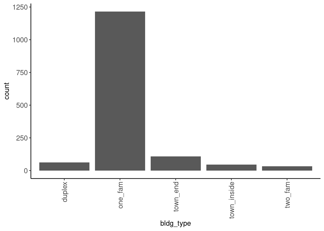

Bar plots can display distributional shape for ordinal variables. May suggest the need for transformations if we later treat the ordinal variable as numeric

See overall_qual. Though it is not very skewed.

data_trn |> plot_bar("overall_qual")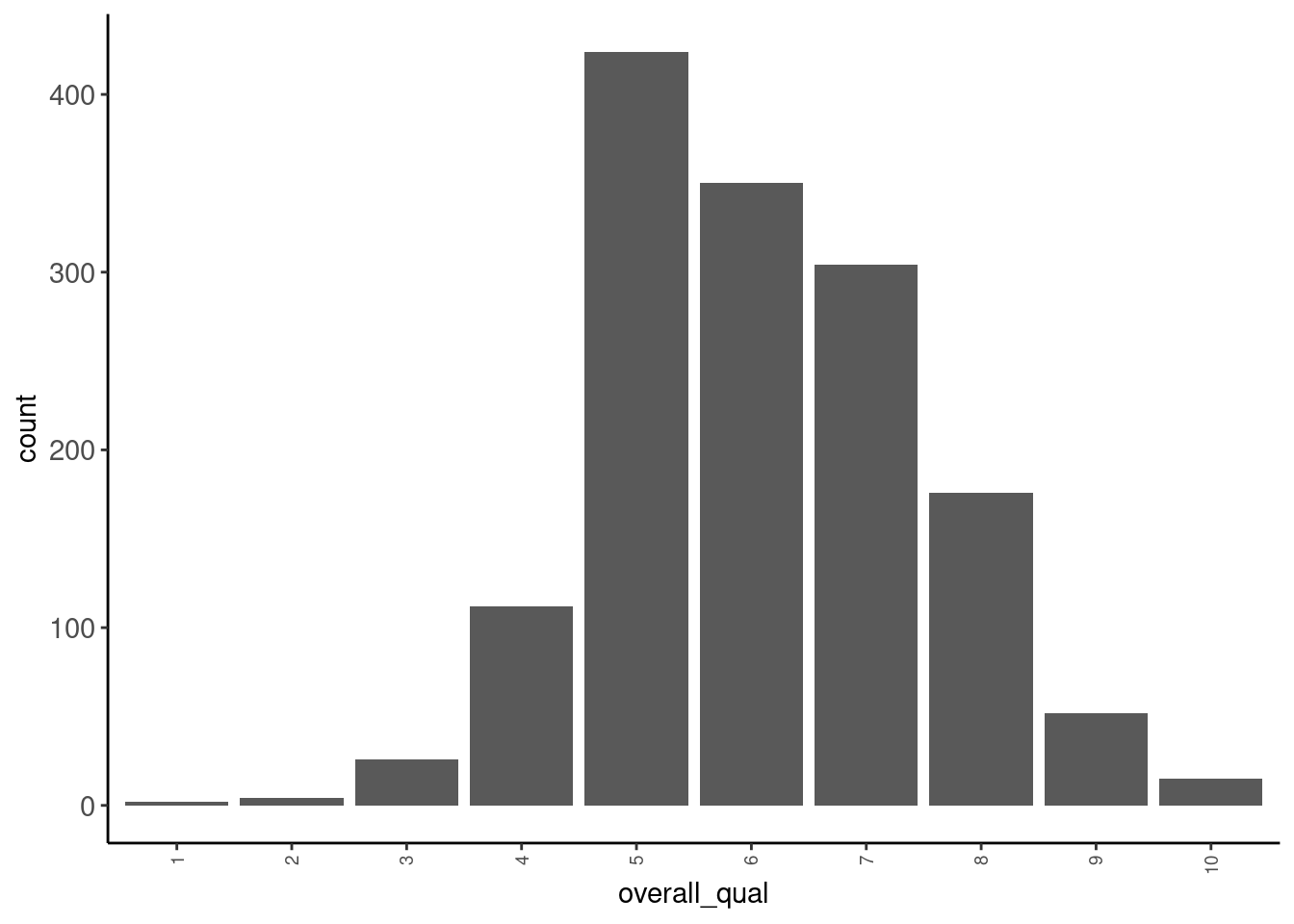

Coding sidebar:

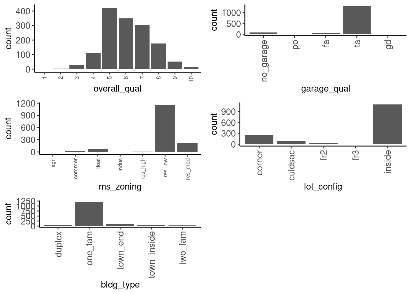
We can make all of our plots iteratively using map() from the `purrr package.

data_trn |> 
1  select(where(is.factor)) |>
2  names() |>
3  map(\(name) plot_bar(df = data_trn, x = name)) |>
4  plot_grid(plotlist = _, ncol = 2)

1: Select only the factor columns
2: Get their names as strings (that is why we use quoted variables in these plot functions
3: Use map() to iterative plot_bar() over every column. (see iteration in Wickham, Çetinkaya-Rundel, and Grolemund (2023))
4: Use plot_grid() from cowplot package to display the list of plots in a grid

2.5.4 Tables for Categorical Variables (Univariate)

We tend to prefer visualizations vs. summary statistics for EDA. However, tables can be useful.

Here is a function that was described in Wickham, Çetinkaya-Rundel, and Grolemund (2023) that we like because

It includes counts and proportions
It includes NA as a category

We have included it in fun_eda.R for your use.

tab <- function(df, var, sort = FALSE) {
  df |>  dplyr::count({{ var }}, sort = sort) |> 
    dplyr::mutate(prop = n / sum(n))
}

Tables can be used to identify responses that have very low frequency and to think about the need to handle missing values

See ms_zoning
May want to collapse low frequency (or low percentage) categories to reduce the number of features needed to represent the predictor

data_trn |> tab(ms_zoning)

# A tibble: 7 × 3
  ms_zoning     n     prop
  <fct>     <int>    <dbl>
1 agri          2 0.00137 
2 commer       13 0.00887 
3 float        66 0.0451  
4 indus         1 0.000683
5 res_high      9 0.00614 
6 res_low    1157 0.790   
7 res_med     217 0.148

We could also view the table sorted if we prefer

data_trn |> tab(ms_zoning, sort = TRUE)

# A tibble: 7 × 3
  ms_zoning     n     prop
  <fct>     <int>    <dbl>
1 res_low    1157 0.790   
2 res_med     217 0.148   
3 float        66 0.0451  
4 commer       13 0.00887 
5 res_high      9 0.00614 
6 agri          2 0.00137 
7 indus         1 0.000683

but could see all this detail with plot as well

data_trn |> plot_bar("ms_zoning")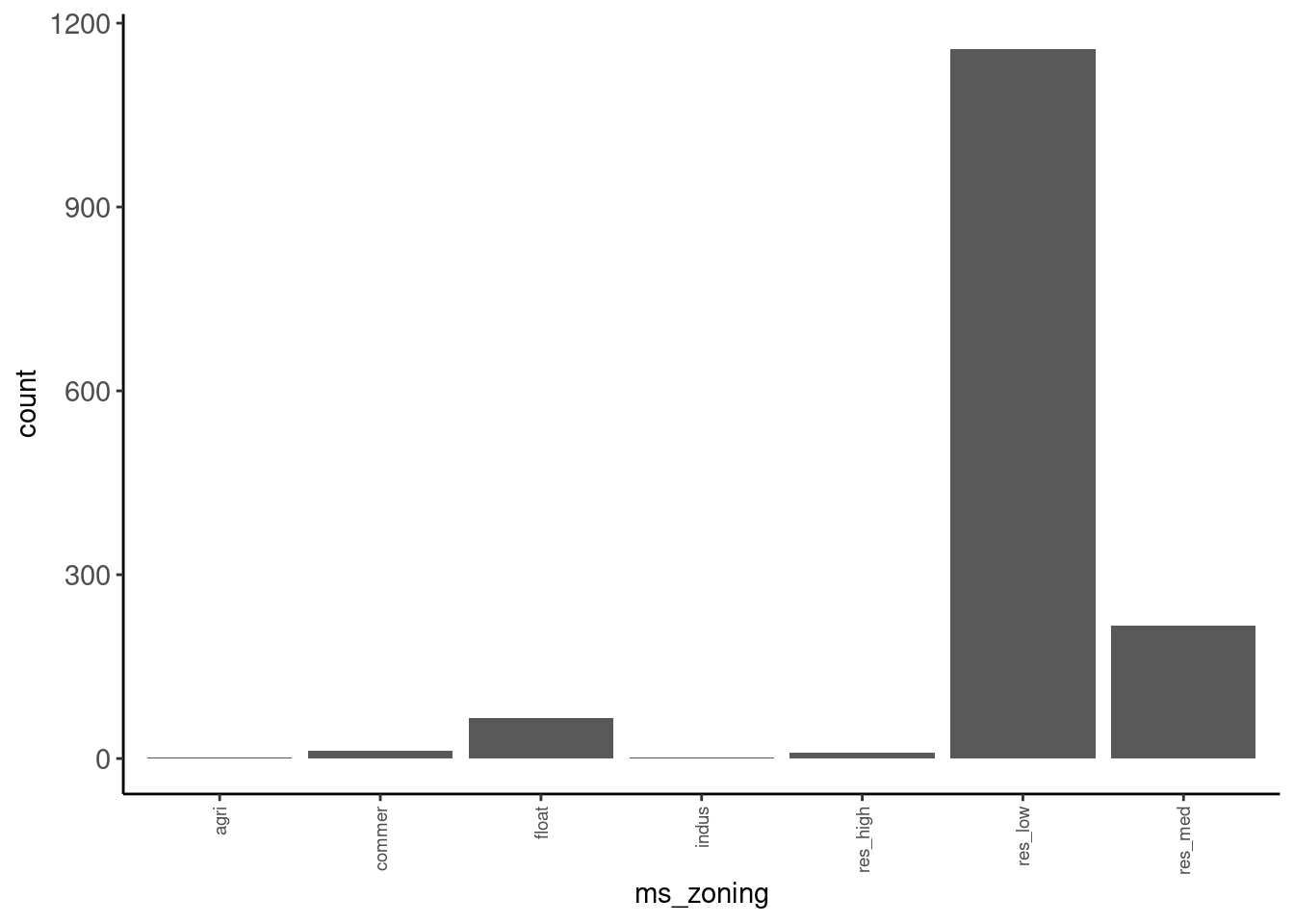

2.5.5 Histograms for Numeric Variables (Univariate)

Histograms are a useful/common visualization for numeric variables

Let’s define a histogram function (included in fun_plots.r)

Bin size should be explored a bit to find best representation
Somewhat dependent on n (my default here is based on this training set)
This is one of the limitations of histograms

plot_hist <- function(df, x, bins = 100){
  df |>
    ggplot(aes(x = .data[[x]])) +
    geom_histogram(bins = bins) +
    theme(axis.text.x = element_text(size = 11),
          axis.text.y = element_text(size = 11))
}

Let’s look at sale_price

It is positively skewed
May suggest units (dollars) are not interval in nature (makes sense)
Could cause problems for some algorithms (e.g., lm) when features are normal

data_trn |> plot_hist("sale_price")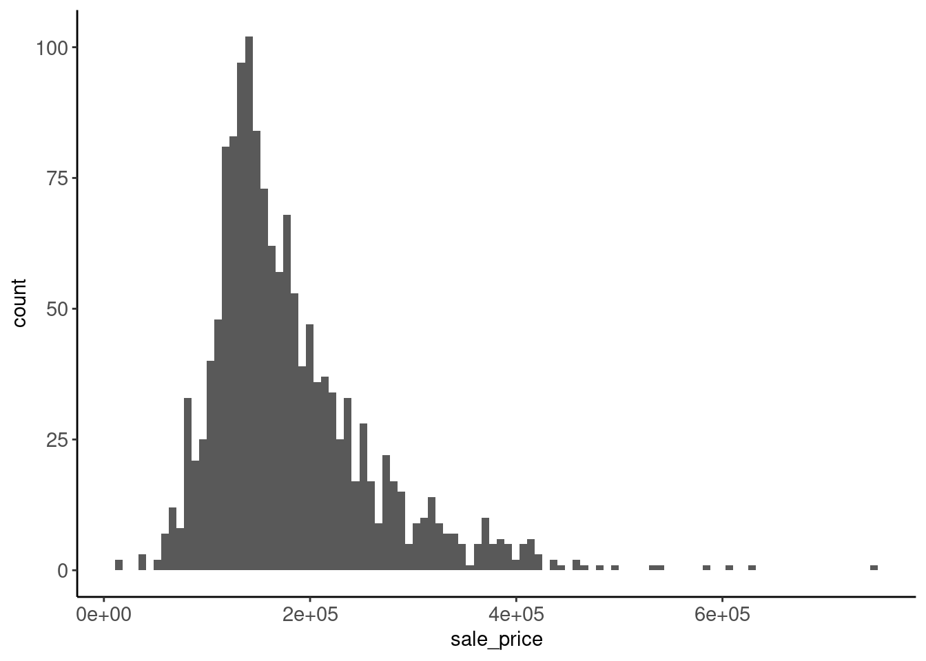

2.5.6 Smoothed Frequency Polygons for Numeric Variables (Univariate)

Frequency polygons are also commonly used

Define a frequency polygon function and use it (included in fun_plots.r)

plot_freqpoly <- function(df, x, bins = 50){
  df |>
    ggplot(aes(x = .data[[x]])) +
    geom_freqpoly(bins = bins) +
    theme(axis.text.x = element_text(size = 11),
          axis.text.y = element_text(size = 11))
}

Bins may matter again

data_trn |> plot_freqpoly("sale_price")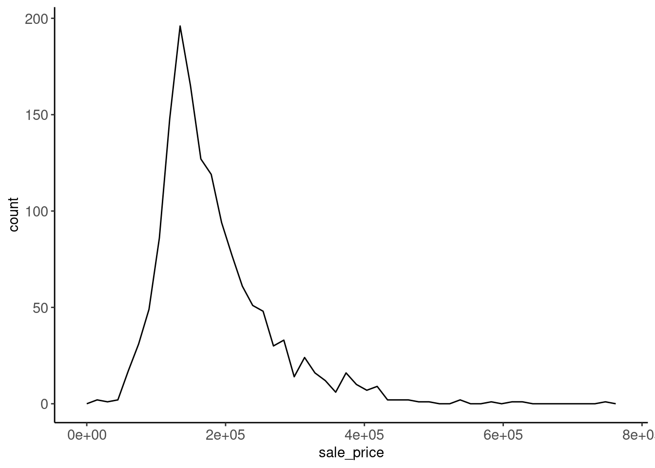

2.5.7 Simple Boxplots for Numeric Variables (Univariate)

Boxplots display

Median as line
25%ile and 75%ile as hinges
Highest and lowest points within 1.5 * IQR (interquartile-range: difference between scores at 25% and 75%iles)
Outliers outside of 1.5 * IQR

Define a boxplot function and use it (included in fun_plots.r)

plot_boxplot <- function(df, x){
  x_label_size <- if_else(skimr::n_unique(df[[x]]) < 7, 11, 7)
  
  df |>
    ggplot(aes(x = .data[[x]])) +
    geom_boxplot() +
    theme(axis.text.y = element_blank(),
          axis.ticks.y = element_blank(),
          axis.text.x = element_text(angle = 90, size = x_label_size, vjust = 0.5, hjust = 1))
}

Here is the plot for sale_price

data_trn |> plot_boxplot("sale_price")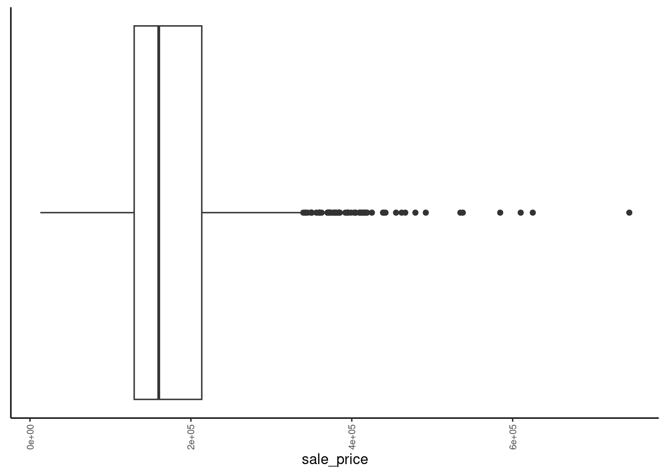

2.5.8 Combined Boxplot and Violin Plots for Numeric Variables (Univariate)

The combination of a boxplot and violin plot is particularly useful

This is our favorite
Get all the benefits of the boxplot
Can clearly see shape of distribution given the violin plot overlay
Can also clearly see the tails

Define a combined plot (included in fun_plots.r)

plot_box_violin <- function(df, x){
  x_label_size <- if_else(skimr::n_unique(df[[x]]) < 7, 11, 7)
  
  df |>
    ggplot(aes(x = .data[[x]])) +
    geom_violin(aes(y = 0), fill = "green", color = NA) +
    geom_boxplot(width = .1, fill = NA, lwd = 1.1, fatten = 1.1) +
    theme(axis.text.y = element_blank(),
          axis.ticks.y = element_blank(),
          axis.title.y = element_blank(),
          axis.text.x = element_text(angle = 90, size = x_label_size, vjust = 0.5, hjust = 1))
}

Here is the plot for sale_price

In this instance, the skew is NOT due to only a few outliers

data_trn |> plot_box_violin("sale_price")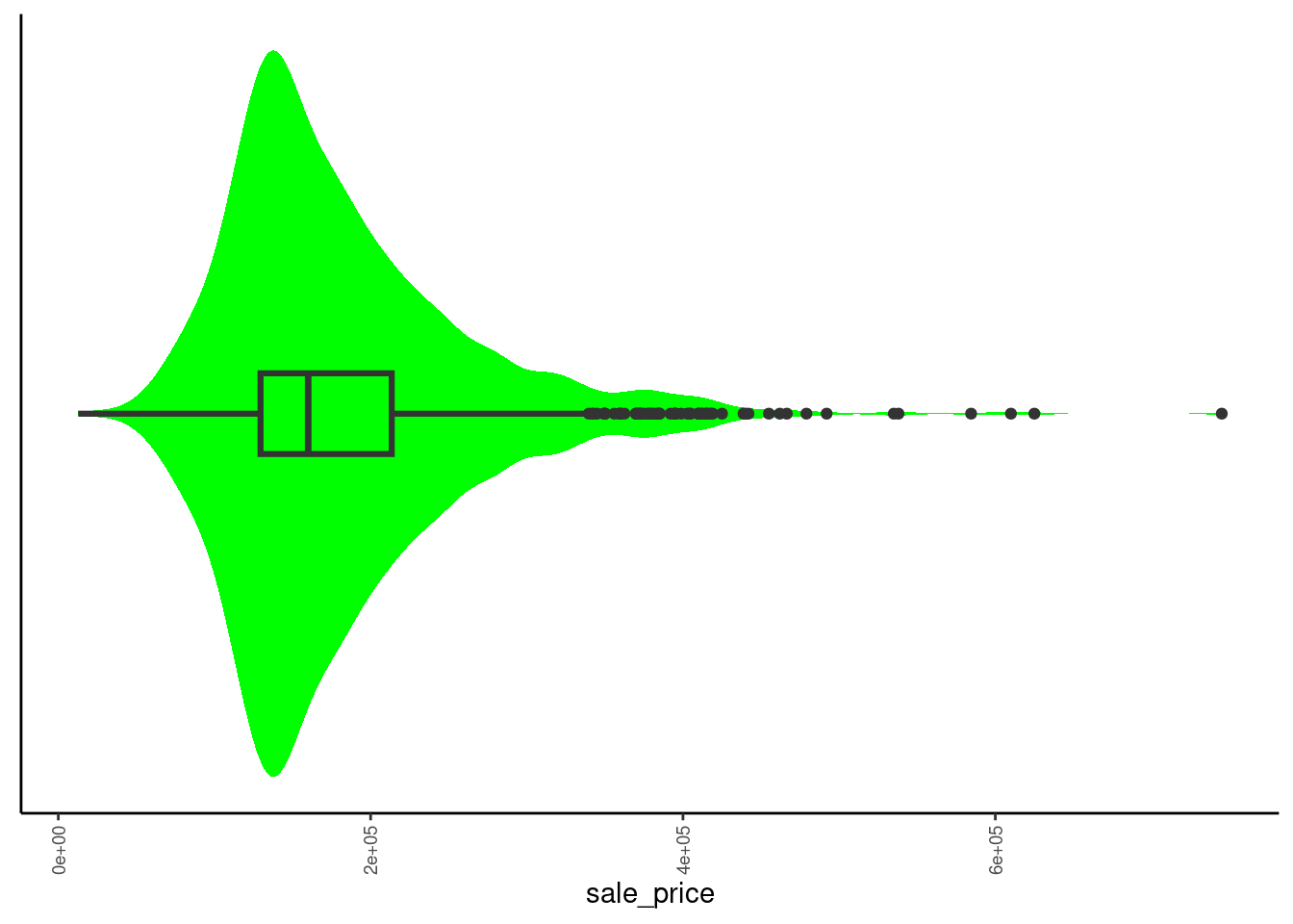

Coding sidebar:

You can make figures for all numeric variables at once using select() and map() as before

data_trn |> 
1  select(where(is.numeric)) |>
  names() |> 
  map(\(name) plot_box_violin(df = data_trn, x = name)) |> 
  plot_grid(plotlist = _, ncol = 2)

1: Now select numeric rather than factor but otherwise same as previous example

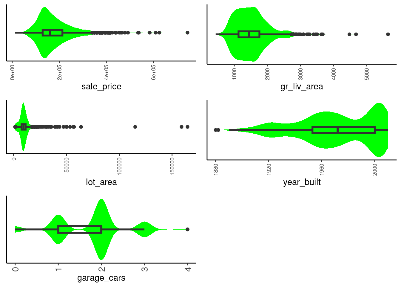
2.5.9 Summary Statistics for Numeric Variables (Univariate)

skim_all() provided all the summary statistics you likely needed for numeric variables

mean & median (p50)
sd & IQR (see difference between p25 and p75)
skew & kurtosis

You can get skim of only numeric variables if you like

data_trn |> 
  skim_all() |> 
  filter(skim_type == "numeric")

Data summary
Name	data_trn
Number of rows	1465
Number of columns	10
_______________________
Column type frequency:
numeric	5
________________________
Group variables	None

Variable type: numeric

skim_variable	n_missing	complete_rate	mean	sd	p0	p25	p50	p75	p100	skew	kurtosis
sale_price	0	1	180696.15	78836.41	12789	129500	160000	213500	745000	1.64	4.60
gr_liv_area	0	1	1506.84	511.44	438	1128	1450	1759	5642	1.43	5.19
lot_area	0	1	10144.16	8177.55	1476	7500	9375	11362	164660	11.20	182.91
year_built	0	1	1971.35	29.65	1880	1953	1972	2000	2010	-0.54	-0.62
garage_cars	1	1	1.78	0.76	0	1	2	2	4	-0.26	0.10

2.5.10 Bivariate Relationships with Outcome

Bivariate relationships with the outcome are useful to detect

Which predictors display some relationship with the outcome
What feature engineering (transformations) might maximize that relationship
Are there any bivariate (model) outliers

Again, we prefer visualizations but summary statistics are also available

2.5.11 Scatterplots for Numeric Variables (Bivariate)

Scatterplots are the preferred visualization when both variables are numeric

Define a scatterplot function (included in fun_plots.r)

add a simple line
add a LOWESS line (Locally Weighted Scatterplot Smoothing)
These lines are useful for considering shape of relationship

plot_scatter <- function(df, x, y){
  df |>
    ggplot(aes(x = .data[[x]], y = .data[[y]])) +
    geom_point() +
    geom_smooth(method = "lm", formula = y ~ x, col = "red") +
    geom_smooth(method = "loess", formula = y ~ x, col = "green") +
    theme(axis.text.x = element_text(size = 11),
          axis.text.y = element_text(size = 11))
}

Let’s consider relationship between gr_liv_area and sale_price

Care most about influential points (both model outlier and leverage)
Can be typically spotted in bivariate plots (but could do more sophisticated assessments)
We might:
- retain as is
- drop
- bring to fence

If bivariate outliers are detected, you should return to cleaning mode to verify that they aren’t result of scoring/coding errors. If they are:

Fix in full dataset
Use same train/test split after fixing

data_trn |> plot_scatter("gr_liv_area", "sale_price")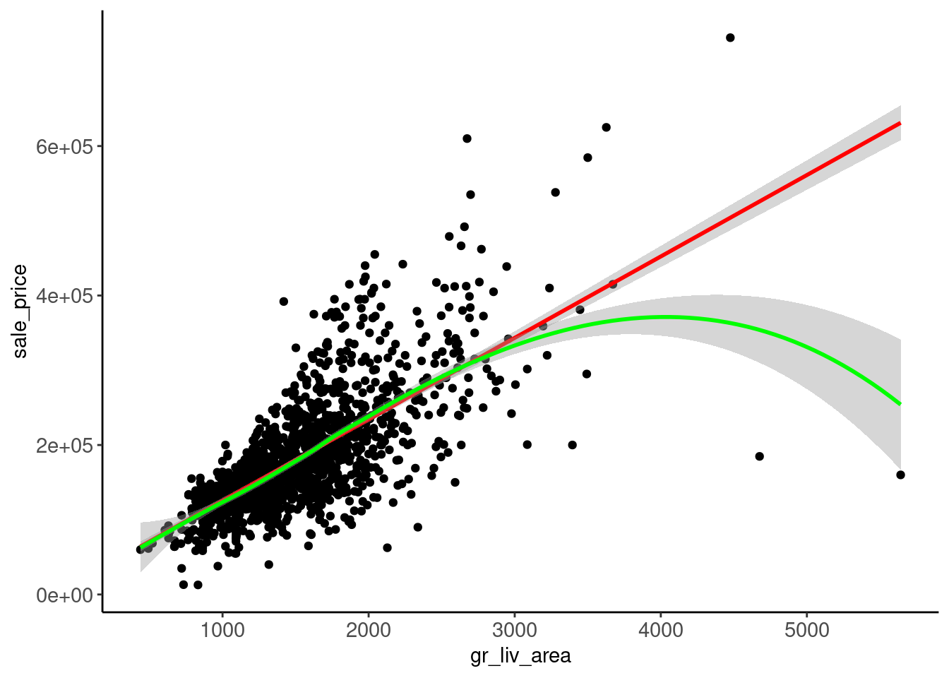

Here is another example where the relationship might be non-linear

data_trn |> plot_scatter("year_built", "sale_price")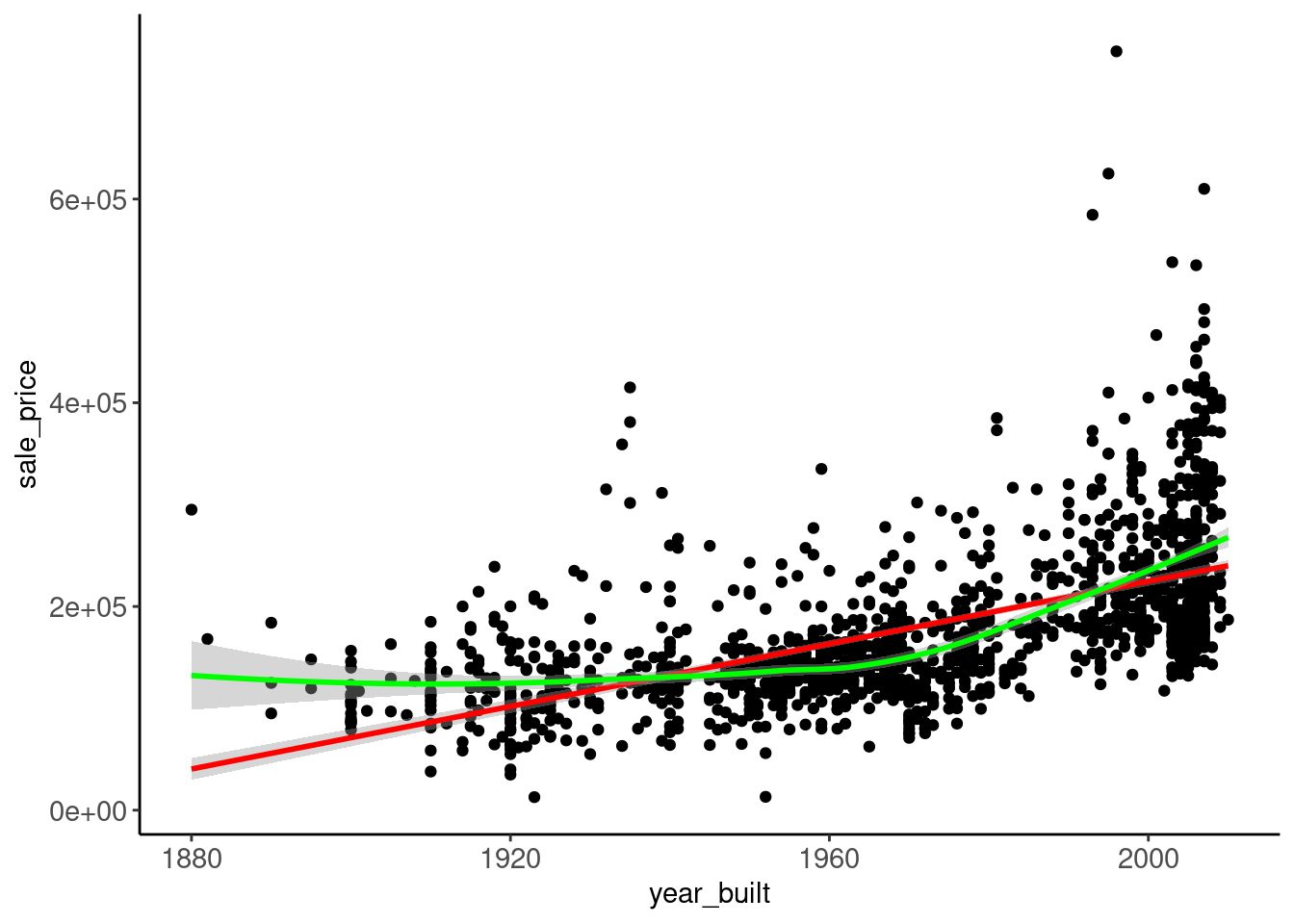

A transformation of sale_price might help the relationship with \(year\_built\) but might hurt gr_liv_area

Maybe need to transform both sale_price and gr_liv_area as both were skewed

This might require some more EDA but here is a start

Quick and temporary Log (base e) of sale_price
This doesn’t seem promising by itself

data_trn |> 
  mutate(sale_price = log(sale_price)) |> 
  plot_scatter("gr_liv_area", "sale_price")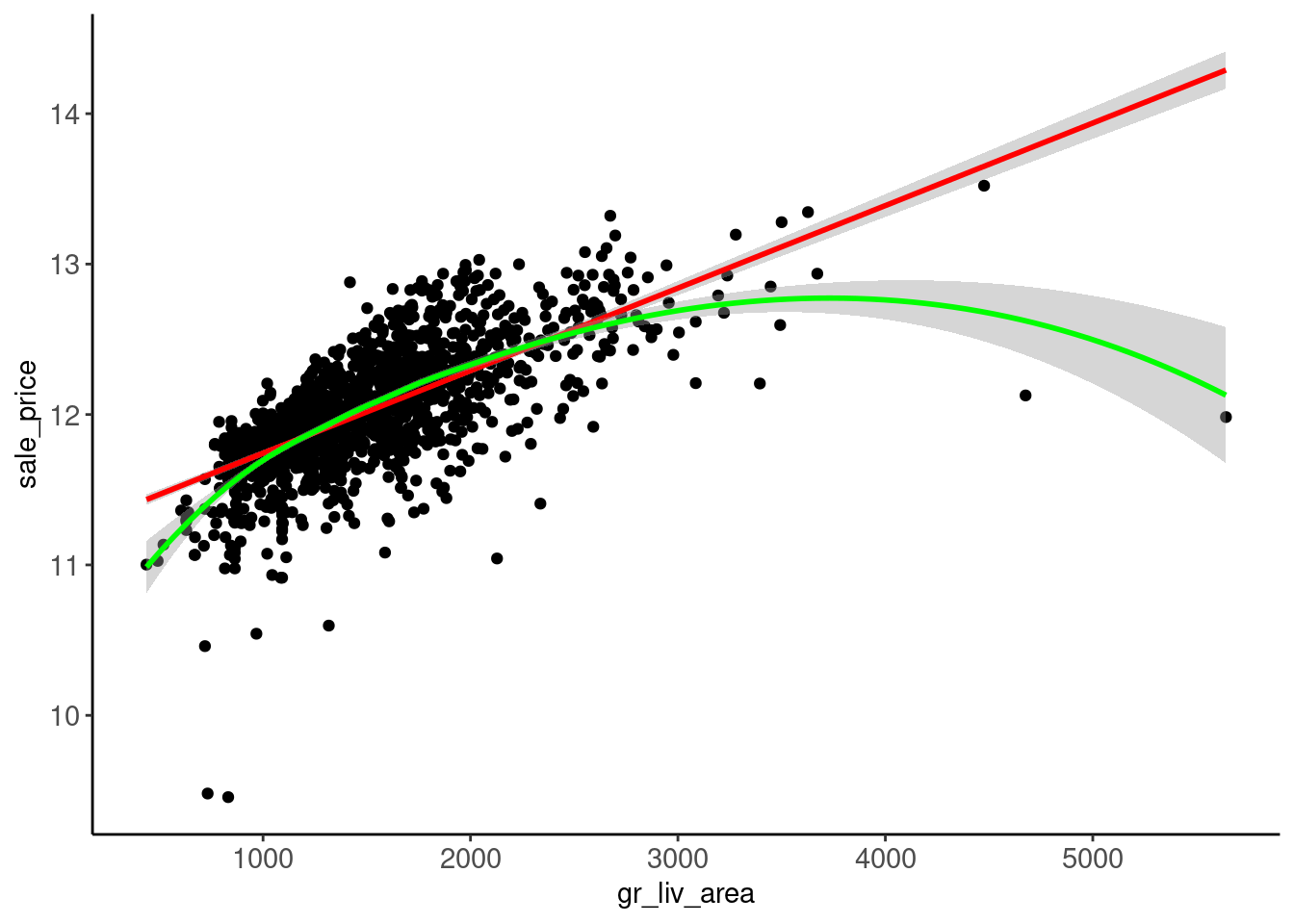

data_trn |> 
  mutate(sale_price = log(sale_price)) |>
  plot_scatter("year_built", "sale_price")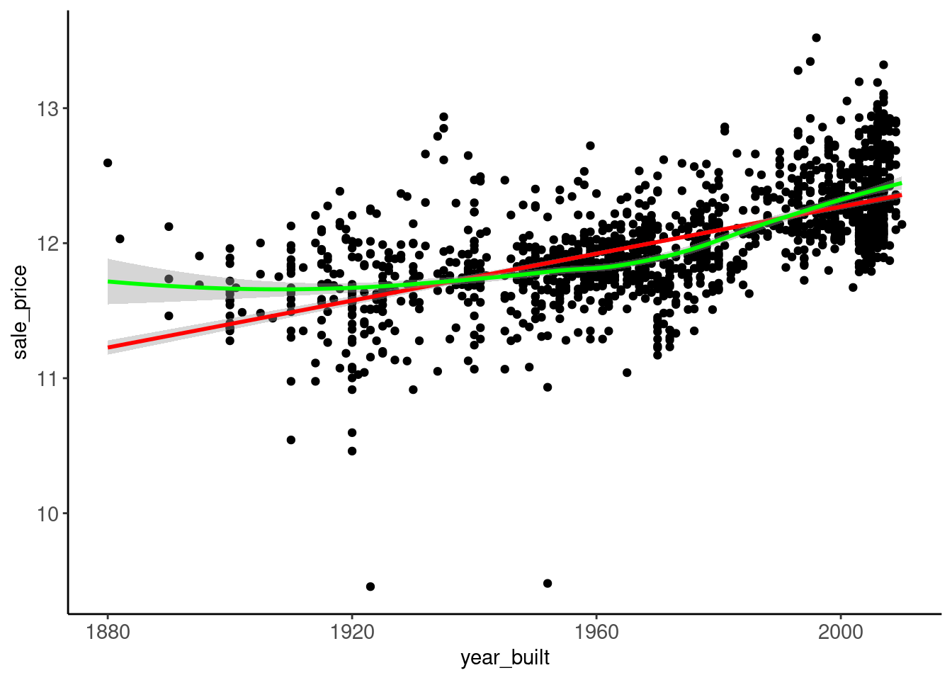

Can make scatterplots for ordinal variables as well

But other (perhaps better) options also exist for this combination of variable classes.
Use as.numeric() to allow for lm and LOWESS lines on otherwise categorical variable

data_trn |> 
  mutate(overall_qual = as.numeric(overall_qual)) |> 
  plot_scatter("overall_qual", "sale_price")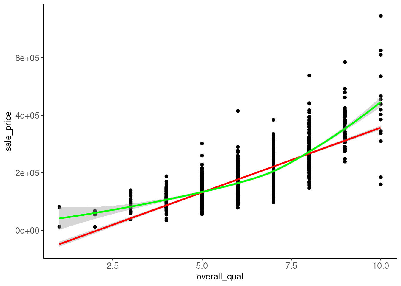

Coding sidebar: Use jitter() with x to help with overplotting

data_trn |> 
  mutate(overall_qual = jitter(as.numeric(overall_qual))) |> 
  plot_scatter("overall_qual", "sale_price")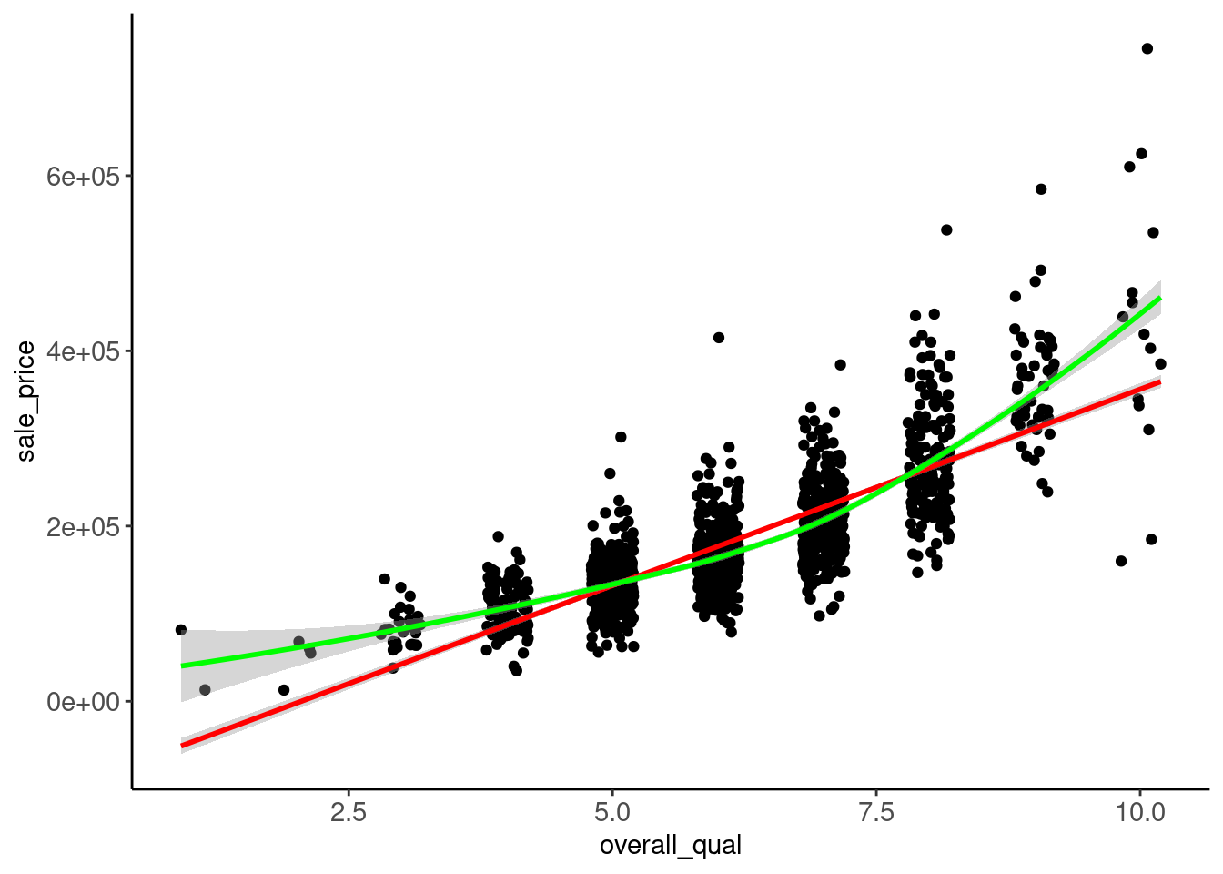

2.5.12 Correlations & Correlation Plots for Numeric Variables (Bivariate)

Correlations are useful summary statistics for numeric variables

Some statistical algorithms are sensitive to high correlations among features (multi-collinearity)

At best, highly correlated features add unnecessary flexibility and can lead to overfitting

We can visualize correlations among predictors/features using corrplot.mixed() from corrplot package

Best for numeric variables
Can include ordinal or two level nominal variables if transformed to numeric
Can include nominal variables with > 2 levels if first transformed appropriately (e.g., dummy features, not demonstrated yet)
Works best with relatively small set of variables

data_trn |> 
  mutate(overall_qual = as.numeric(overall_qual),
         garage_qual = as.numeric(garage_qual)) |> 
  select(where(is.numeric)) |> 
  cor(use = "pairwise.complete.obs") |> 
1  corrplot::corrplot.mixed()

1: Note use of namespace (corrplot::corrplot.mixed()) to call this function from corrplot package

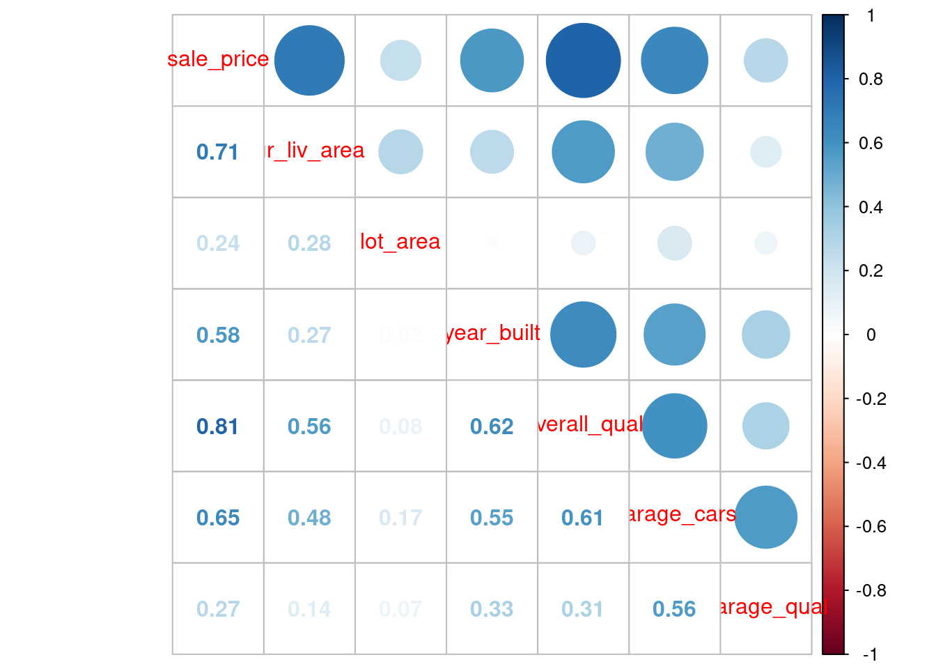
2.5.13 Grouped Box + Violin Plots for Categorical and Numeric (Bivariate)

A grouped version of the combined box and violin plot is our preferred visualization for relationship between categorical and numeric variables (included in fun_plots.r)

Often best when feature is categorical and outcome is numeric but can reverse
Can use with both nominal and ordinal categorical variable
Wickham, Çetinkaya-Rundel, and Grolemund (2023) also describes use of grouped frequency polygons for this combination of variable classes

plot_grouped_box_violin <- function(df, x, y){
  x_label_size <- if_else(skimr::n_unique(df[[x]]) < 7, 11, 7)
  
  df |>
    ggplot(aes(x = .data[[x]], y = .data[[y]])) +
    geom_violin(fill = "green", color = NA) +
    geom_boxplot(width = .1, fill = NA, lwd = 1.1, fatten = 1.1) +
    theme(axis.text.x = element_text(angle = 90, size = x_label_size, 
                                     vjust = 0.5, hjust = 1),
          axis.text.y = element_text(size = 11))
}

Here is the relationship between overall_qual and sale_price

Tend to prefer this over the scatterplot (with as.numeric()) for ordinal variables
Increasing spread of sale_price at higher levels of overall_qual is clearer in this plot

data_trn |> plot_grouped_box_violin("overall_qual", "sale_price")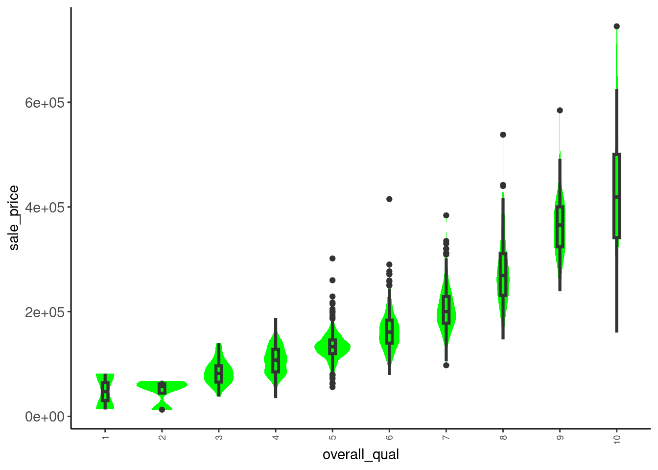

Here is a grouped box + violin with a nominal variable

More variation and skew in sale_price for one family homes (additional features, moderators?)
Position of townhouse (interior vs. exterior) seems to matter (don’t collapse?)

data_trn |> plot_grouped_box_violin("bldg_type", "sale_price")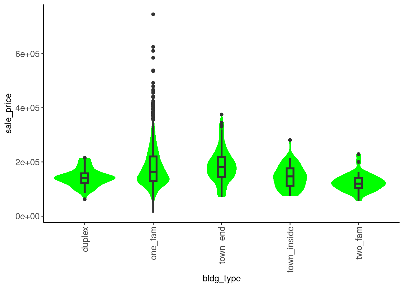

When we have a categorical predictor and a numeric outcome, we often want to see both the relationship between the variables AND the variability on the categorical variable alone.

We like this combined plot enough when doing EDA to provide a specific function (included in fun_plots.r)!

It is our go to for understanding the potential effect of a categorical predictor

plot_categorical <- function(df, x, y, ordered = FALSE){
  if (ordered) {
    df <- df |>
      mutate(!!x := fct_reorder(.data[[x]], .data[[y]]))
  }
  
  x_label_size <- if_else(skimr::n_unique(df[[x]]) < 7, 11, 7)
  
  p_bar <- df |>
    ggplot(aes(x = .data[[x]])) +
    geom_bar()  +
    theme(axis.text.x = element_text(angle = 90, size = x_label_size, 
                                     vjust = 0.5, hjust = 1),
          axis.text.y = element_text(size = 11))
  
  p_box <- df |>
    ggplot(aes(x = .data[[x]], y = .data[[y]])) +
    geom_violin(fill = "green", color = NA) +
    geom_boxplot(width = .1, fill = NA, lwd = 1.1, fatten = 1.1) +
    theme(axis.text.x = element_text(angle = 90, size = x_label_size, 
                                     vjust = 0.5, hjust = 1),
          axis.text.y = element_text(size = 11))
  
  return(list(p_bar, p_box))
}

sale_price by bldg_type

data_trn |> plot_categorical("bldg_type", "sale_price") |> 
  plot_grid(plotlist = _, ncol = 1)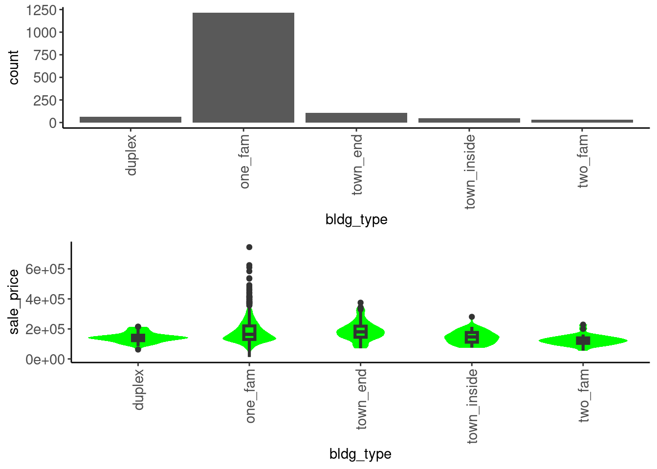

2.5.14 Stacked Barplots for Categorical (Bivariate)

Stacked Barplots:

Can be useful with both nominal and ordinal variables
Can create with either raw counts or percentages.
- Displays different perspective (particularly with uneven distributions across levels)
- Depends on your question
Often, you will place the outcome on the x-axis and the feature is coded by fill

plot_grouped_barplot_count <- function(df, x, y){
  x_label_size <- if_else(skimr::n_unique(df[[x]]) < 7, 11, 7)
  
  df |>
    ggplot(aes(x = .data[[y]], fill = .data[[x]])) +
    geom_bar(position = "stack") +
    theme(axis.text.x = element_text(angle = 90, size = x_label_size, 
                                     vjust = 0.5, hjust = 1),
          axis.text.y = element_text(size = 11))
}

plot_grouped_barplot_percent <- function(df, x, y){
  x_label_size <- if_else(skimr::n_unique(df[[x]]) < 7, 11, 7)
  
  df |>
    ggplot(aes(x = .data[[y]], fill = .data[[x]])) +
    geom_bar(position = "fill") +
    labs(y = "Proportion") +
    theme(axis.text.x = element_text(angle = 90, size = x_label_size, 
                                     vjust = 0.5, hjust = 1),
          axis.text.y = element_text(size = 11))
}

For example, if we wanted to learn about how bldg_type varies by lot_config, see these plots

data_trn |> plot_grouped_barplot_count("lot_config", "bldg_type")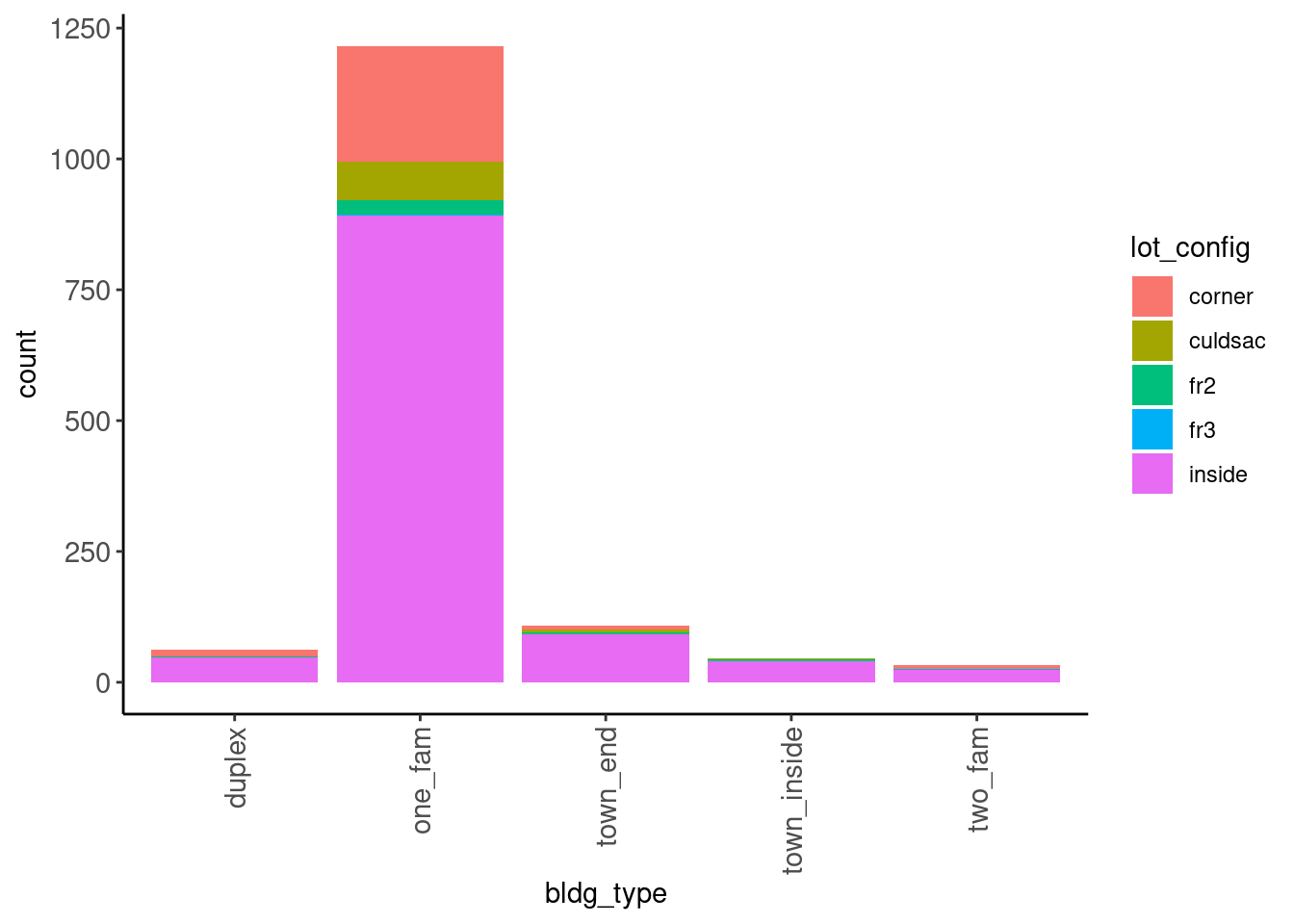

data_trn |> plot_grouped_barplot_percent("lot_config", "bldg_type")

May want to plot both ways

data_trn |> plot_grouped_barplot_percent("lot_config", "bldg_type")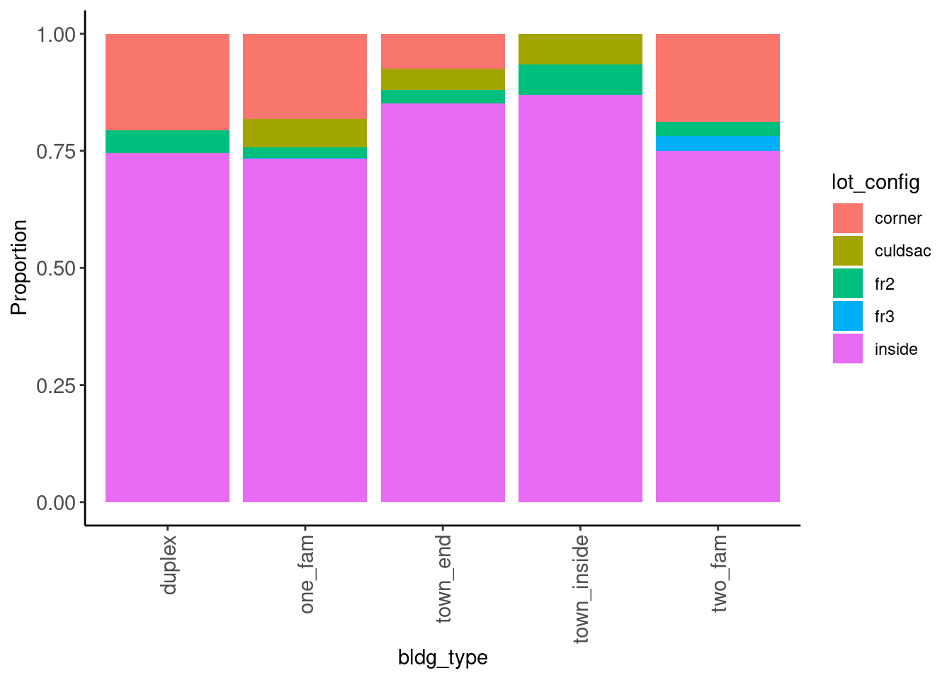

data_trn |> plot_grouped_barplot_percent("bldg_type", "lot_config")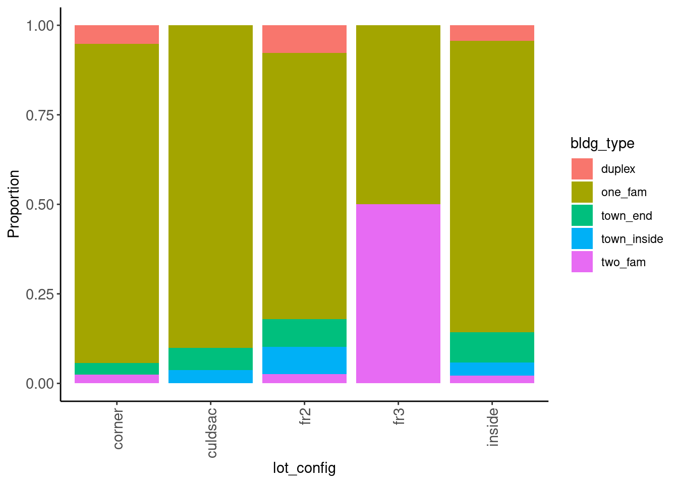

2.5.15 Tile Plot for Ordinal Categorical (Bivariate)

Tile plots may be useful if both categorical variables are ordinal

plot_tile <- function(df, x, y){
  df |>
    count(.data[[x]], .data[[y]]) |>
    ggplot(aes(x = .data[[x]], y = .data[[y]])) +
    geom_tile(mapping = aes(fill = n))
}

data_trn |> plot_tile("overall_qual", "garage_qual")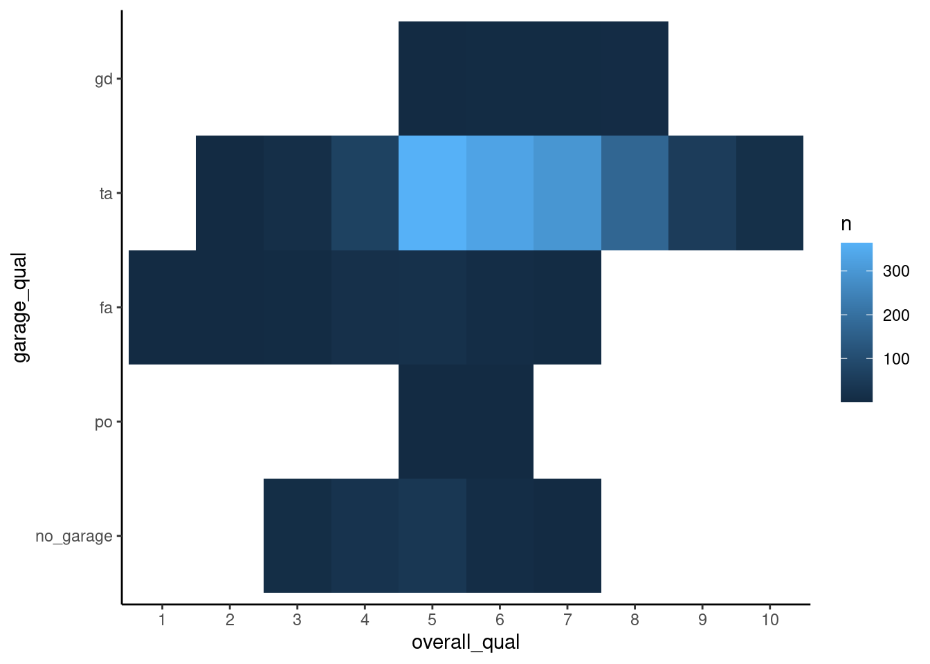

You might also consider a scatterplot with jitter in this instance

data_trn |> 
  mutate(overall_qual = jitter(as.numeric(overall_qual)),
         garage_qual = as.numeric(garage_qual)) |> 
  plot_scatter("overall_qual", "garage_qual")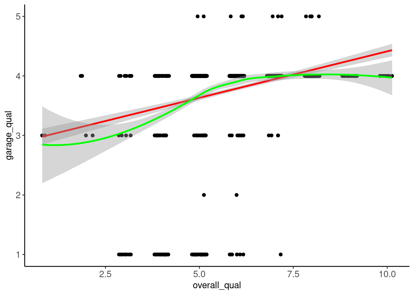

2.5.16 Two-way Tables for Categorical Variables (Bivariate)

Two-way tables are sometimes a useful summary statistic for two categorical variables. We can use a 2-variable form of the tab function, tab2(), from my function scripts for this

For example, the relationship between bldg_type and lot_config

data_trn |> tab2(bldg_type, lot_config)

   bldg_type corner culdsac fr2 fr3 inside
      duplex     13       0   3   0     47
     one_fam    221      73  29   1    892
    town_end      8       5   3   0     92
 town_inside      0       3   3   0     40
     two_fam      6       0   1   1     24

2.6 Working with Recipes

Recipes are used for feature engineering in tidymodels using the recipes package

Used for transforming raw predictors into features used in our models
Describes all steps to make feature matrix. For example:
- Transforming factors into “dummy” features if needed
- Linear and non-linear transformations (e.g., log, box-cox)
- Polynomials and interactions (i.e., x1 * x1 or x1 * x2)
- Missing value imputations
Proper use of recipes is an important tool to prevent data leakage between train and either validation or test.
Recipes use only information from the training set in all feature engineering
Consider example of standardizing x1 for a feature in train vs. validation and test. Must use mean and sd from TRAIN to standardize x1 in train, validate, and test. VERY IMPORTANT.

We use recipes in a two step process - prep() and bake()

“Prepping” a recipe involves calculating any statistics needed for the transformations that will be applied to engineer features (e.g., mean and standard deviation to normalize a numeric variable).
- Prepping is done with the prep() function.
- Prepping is always done only with training data. A “prepped” recipe does not derive any statistics from validation or test sets.
“Baking” is the process of calculating the features
- Baking is done with the bake() function.
- We used our prepped recipe when we bake.
- Whereas we only prep a recipe with training data, we can use a prepped recipe to bake features from any dataset (training, validation, or test).

We will work with recipes extensively when model building starting in unit 3

For now, we will only use the recipe to indicate roles as a gentle introduction.

We will expand on this recipe in unit 3

Recipe syntax is very similar to generic tidyverse syntax (created by same group)

Actually a subset of tidyverse functions
Less flexible/powerful but focused on our needs and easier to learn
You will eventually know both

Recipes are used in Modeling scripts (which is a third type of script after cleaning and modeling EDA scripts)

Lets reload training again to pretend we are starting a new script

 data_trn <- read_csv(file.path(path_data, "ames_clean_class_trn.csv"), 
                      col_types = cols()) |> 
1  class_ames() |>
  glimpse()

1: Remember our function for classing!

Rows: 1,465
Columns: 10
$ sale_price   <dbl> 105000, 126000, 115000, 120000, 99500, 112000, 122000, 12…
$ gr_liv_area  <dbl> 896, 882, 864, 836, 918, 1902, 900, 1225, 1728, 858, 1306…
$ lot_area     <dbl> 11622, 8400, 10500, 2280, 7892, 8930, 9819, 9320, 13260, …
$ year_built   <dbl> 1961, 1970, 1971, 1975, 1979, 1978, 1967, 1959, 1962, 195…
$ overall_qual <fct> 5, 4, 4, 7, 6, 6, 5, 4, 5, 5, 3, 5, 4, 5, 3, 5, 2, 6, 5, …
$ garage_cars  <dbl> 1, 2, 0, 1, 1, 2, 1, 0, 0, 0, 0, 1, 2, 2, 1, 1, 2, 2, 1, …
$ garage_qual  <fct> ta, ta, no_garage, ta, ta, ta, ta, no_garage, no_garage, …
$ ms_zoning    <fct> res_high, res_low, res_low, res_low, res_low, res_med, re…
$ lot_config   <fct> inside, corner, fr2, fr2, inside, inside, inside, inside,…
$ bldg_type    <fct> one_fam, one_fam, one_fam, town_inside, town_end, duplex,…

Recipes can be used to indicate the outcome and predictors that will be used in the model

Can use . to indicate all predictors
- Currently, our preferred method for larger data sets
- We can exclude some predictors later by changing their role, removing them with a later recipe step (\(step\_rm()\)), or specifying a more precise formula when we fit the model
- See Roles in Recipes for more info
Can use specific names of predictors along with \(+\)
- This is our preferred method when we have a smaller set of predictors (We will show you both approaches)
- e.g., sale_price ~ lot_area + year_built + overall_qual
Do NOT indicate interactions here
- All predictors are combined with +
- Interactions are specified by a later explicit feature engineering step

rec <- recipe(sale_price ~ ., data = data_trn)

rec

── Recipe ──────────────────────────────────────────────────────────────────────

── Inputs

Number of variables by role

outcome:   1
predictor: 9

summary(rec)

# A tibble: 10 × 4
   variable     type      role      source  
   <chr>        <list>    <chr>     <chr>   
 1 gr_liv_area  <chr [2]> predictor original
 2 lot_area     <chr [2]> predictor original
 3 year_built   <chr [2]> predictor original
 4 overall_qual <chr [3]> predictor original
 5 garage_cars  <chr [2]> predictor original
 6 garage_qual  <chr [3]> predictor original
 7 ms_zoning    <chr [3]> predictor original
 8 lot_config   <chr [3]> predictor original
 9 bldg_type    <chr [3]> predictor original
10 sale_price   <chr [2]> outcome   original

2.6.1 Prepping and Baking a Recipe

Let’s make a feature matrix from the training set

There are two discrete (and important) steps

prep()
bake()

First we prep the recipe using the training data

1rec_prep <- rec |>
2  prep(training = data_trn)

1: We start by prepping our raw/original recipe (rec)
2: We use the prep() function on on the training data. Recipes are ALWAYS prepped using training data. This makes sure that are recipes will always only use information from the training set when making features for any subsequent dataset. As part of the prepping process, prep() calculates and saves the features for the training data for later use

Second, we bake the training data using this prepped recipe to get a feature matrix from it.

We set new_data = NULL because don’t need features for new data. Instead, we want features from the training data that were used to prep the recipe

feat_trn <- rec_prep |> 
  bake(new_data = NULL)

Finally, we should generally at least glimpse and/or skim (and typically do some more EDA) on our features to make sure our recipe is doing what we expect.

glimpse

feat_trn |> glimpse()

Rows: 1,465
Columns: 10
$ gr_liv_area  <dbl> 896, 882, 864, 836, 918, 1902, 900, 1225, 1728, 858, 1306…
$ lot_area     <dbl> 11622, 8400, 10500, 2280, 7892, 8930, 9819, 9320, 13260, …
$ year_built   <dbl> 1961, 1970, 1971, 1975, 1979, 1978, 1967, 1959, 1962, 195…
$ overall_qual <fct> 5, 4, 4, 7, 6, 6, 5, 4, 5, 5, 3, 5, 4, 5, 3, 5, 2, 6, 5, …
$ garage_cars  <dbl> 1, 2, 0, 1, 1, 2, 1, 0, 0, 0, 0, 1, 2, 2, 1, 1, 2, 2, 1, …
$ garage_qual  <fct> ta, ta, no_garage, ta, ta, ta, ta, no_garage, no_garage, …
$ ms_zoning    <fct> res_high, res_low, res_low, res_low, res_low, res_med, re…
$ lot_config   <fct> inside, corner, fr2, fr2, inside, inside, inside, inside,…
$ bldg_type    <fct> one_fam, one_fam, one_fam, town_inside, town_end, duplex,…
$ sale_price   <dbl> 105000, 126000, 115000, 120000, 99500, 112000, 122000, 12…

skim

feat_trn |> skim_all()

Data summary
Name	feat_trn
Number of rows	1465
Number of columns	10
_______________________
Column type frequency:
factor	5
numeric	5
________________________
Group variables	None

Variable type: factor

skim_variable	complete_rate	n_unique	top_counts
overall_qual	1	10	5: 424, 6: 350, 7: 304, 8: 176
garage_qual	1	5	ta: 1312, no_: 81, fa: 57, gd: 13
ms_zoning	1	7	res: 1157, res: 217, flo: 66, com: 13
lot_config	1	5	ins: 1095, cor: 248, cul: 81, fr2: 39
bldg_type	1	5	one: 1216, tow: 108, dup: 63, tow: 46

Variable type: numeric

skim_variable	n_missing	complete_rate	mean	sd	p0	p25	p50	p75	p100	skew	kurtosis
gr_liv_area	0	1	1506.84	511.44	438	1128	1450	1759	5642	1.43	5.19
lot_area	0	1	10144.16	8177.55	1476	7500	9375	11362	164660	11.20	182.91
year_built	0	1	1971.35	29.65	1880	1953	1972	2000	2010	-0.54	-0.62
garage_cars	1	1	1.78	0.76	0	1	2	2	4	-0.26	0.10
sale_price	0	1	180696.15	78836.41	12789	129500	160000	213500	745000	1.64	4.60

We can now use our features from training to train models, but that will take place in the next unit!

We could also use the prepped recipe to bake validation or test data to evaluate trained models. That too will happen in the next unit!

2.7 Discussion Topics

House keeping
- Unit 2 solutions
- Course evals for extra credit (to quiz score)!
- Unit 3 homework
  - test set predictions
  - free lunch!
- Questions to all three of us
- An attempt at a reprex is generally expected now for code help
Quiz review
Student Questions
- great questions!
- write them down as you read and watch lectures
- not all questions will fit (slack as an alternative for follow-up)

# Possible topics

Review
- Goal is to develop model that closely approximates DGP
- Goal is to evaluate (estimate) how close our model is to the DGP (how much error) with as little error as possible
- Bias, overfitting/variance for any estimate (model and performance of model)
- candidate model configurations
- fit, select, evaluate
- training, validation, test
Review: 2.2.1 Stages of Data Analysis and Model Development
Best practices (discuss quickly)
- csv for data sharing, viewing, git (though be careful with data in github or other public repo!)
- variable values saved as text when nominal and ordinal (self-documenting)
- Create data dictionary - Documentation is critical!!
- snake_case for variables and self-documenting names (systematic names too)
Review: 2.3.1 Data Leakage Issues
- Review section in webbook
- Cleaning EDA is done with full dataset (but univariate). Very limited (variable names, values, find errors)
- Modeling EDA is only done with a training set (or even “eyeball” sample) - NEVER use validate or test set
- Never estimate anything with full data set (e.g., missing values, standardize, etc)
- Use recipes, prep (all estimation) with held in data than bake the appropriate set
- Put test aside
- You work with validation but never explore with validation (will still catch leakage with test but will be mislead to be overly optimistic and spoil test)
Functions sidenote - fun_modeling.R on github
Review: 2.4.2 Prepping and Baking a Recipe
- Review section in web book
- prep always with held in data, bake with held in & out data.
EDA for modeling
- limitless, just scratched the surface
- Differs some based on dimenstionality of dataset
- Learning about DGP
  - understand univariate distributions, frequencies
  - bivariate relationships
  - interactions (3 or more variables)
  - patterns in data
Extra topics, time permitting

8.1. Missing data

- Exclude vs. Impute in training data.  Outcomes?
- How to impute
- Missing in validate or test (can't exclude?). Exclude cases with missing outcomes.

8.2. Outliers - Drop or fix errors! - Goal is always to estimate DGP - Exclude - Retain - Bring to fence - Don’t exclude/change outcome in validate/test

8.3. Issues with high dimensionality

- Hard to do predictor level EDA
- Common choices (normality transformations)
- observed vs. predicted plots
- Methods for automated variable selection (glmnet)

8.4. Distributional Shape

- Measurement issues (interval scale)
- Implications for relationships with other variables
- Solutions?

8.5. Linearity vs. More Complex Relationships

- Transformations
- Choice of statistical algorithm
- Do you need a linear model?

8.6. Interactions

- Domain expertise
- Visual options for interactions
- But what do do with high dimensional data?
- Explanatory vs. prediction goals (algorithms that accommodate interactions)

8.7. How to handle all of these decisions in the machine learning framework

- Goal is to develop a model that most closely approximates the DGP
- How does validation and test help this?
- Preregistration?
  - Pre-reg for performance metric, resampling method   
  - Use of resampling for other decisions
  - Use of resampling to find correct model to test explanatory goals

8.8. Model Assumptions

- Why do we make assumptions?
  - Inference
  - Flexibility wrt DGP

Wickham, Hadley. 2019. Advanced r. 2nd ed. https://adv-r.hadley.nz/.

Wickham, Hadley, Çetinkaya-Rundel Mine, and Garrett Grolemund. 2023. R for Data Science: Visualize, Model, Transform, and Import Data. 2nd ed. https://r4ds.hadley.nz/.