9 Advanced Models: Decision Trees, Bagging Trees, and Random Forest

9.1 Overview of Unit

9.1.1 Learning Objectives

Decision trees
Bagged trees
How to bag models and the benefits
Random Forest
How Random Forest extends bagged trees
Feature interpretation with decision tree plots

9.1.2 Readings

James et al. (2023) Chapter 8, Tree Based Methods; pp 327 - 352

In addition, much of the content from this unit has been drawn from four chapters in a book called Hands On Machine Learning In R. It is a great book and I used it heavily (and at times verbatim) b/c it is quite clear in its coverage of these algorithms. If you want more depth, you might read chapters 9-12 from this book as a supplement to this unit in our course.

Post questions to the readings channel in Slack

9.1.3 Lecture Videos

Lecture 1: Decision Trees ~ 30 mins
Lecture 2: Decision Trees in Ames ~ 20 mins
Lecture 3: Bagged Treesi ~ 10 mins
Lecture 4: Bagged Trees in Ames ~ 6 mins
Lecture 5: Random Forest ~ 16 mins

Post questions to the video-lectures channel in Slack

9.1.4 Coding Assignment

Post questions to application-assignments Slack channel

Submit the application assignment here and complete the unit quiz by 8 pm on Wednesday, March 20th

9.2 Decision Trees

Tree-based statistical algorithms:

Are a class of flexible, nonparametric algorithms
Work by partitioning the feature space into a number of smaller non-overlapping regions with similar responses by using a set of splitting rules
Make predictions by assigning a single prediction to each of these regions
Can produce simple rules that are easy to interpret and visualize with tree diagrams
Typically lack in predictive performance compared to other common algorithms
Serve as base learners for more powerful ensemble approaches

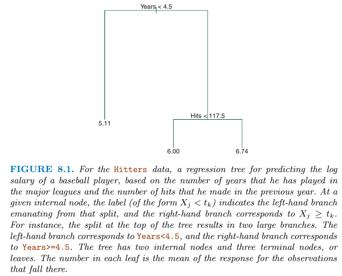
In figure 8.1 from James et al. (2023), they display a simple tree to predict log(salary) using years in the major league and hits from the previous year

This tree only has a depth of two (there are only two levels of splits)

years < 4.5
hits < 117.5

This results in three regions

years < 4.5
years >= 4.5 & hits < 117.5
years >= 4.5 & hits >= 117.5

A single value for salary is predicted for each of these three regions

Decision trees are very interpretable. How we make decisions?

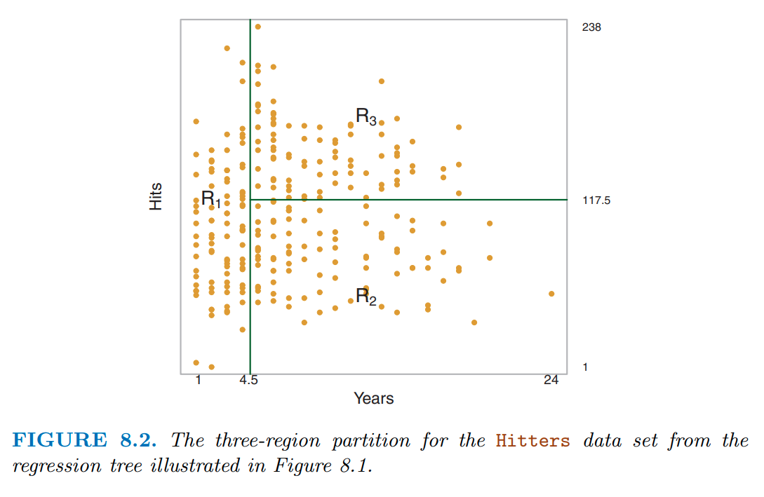
You can see these regions more clearly in the two-dimensional feature space displayed in figure 8.2

Notice how even with a limited tree depth of 2, we can already get a complex partitioning of the feature space.

Decision trees can encode complex decision boundaries (and even more complex than this as tree depth increases)

There are many methodologies for constructing decision trees but the most well-known is the classification and regression tree (CART) algorithm proposed in Breiman (1984)

This algorithm is implemented in the rpart package and this is the engine we will use in tidymodels for decision trees (and bagged trees - a more advance ensemble method)
The decision tree partitions the training data into homogeneous subgroups (i.e., groups with similar response values)
These subgroups are called nodes
The nodes are formed recursively using binary partitions by asking simple yes-or-no questions about each feature (e.g., are years in major league < 4.5?)
This is done a number of times until a suitable stopping criteria is satisfied, e.g.,
- a maximum depth of the tree is reached
- minimum number of remaining observations is available in a node
After all the partitioning has been done, the model predicts a single value for each region
- mean response among all observations in the region for regression problems
- majority vote among all observations in the region for classification problems
- probabilities (for classification) can be obtained using the proportion of each class within the region

The bottom left panel in Figure 8.3 shows a slightly more complicated tree with depth = 3 for two arbitrary predictors (x1 and x2)

The right column shows a representation of the regions formed by this tree (top) and a 3D representation that includes predictions for y (bottom)

The top left panel displays a set of regions that is NOT possible using binary recursive splitting. This makes the point that there are some patterns in the data that cannot be accommodated well by decision trees

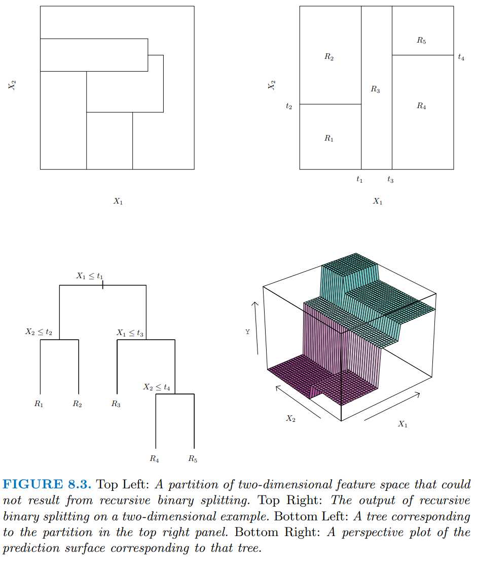
Figure 8.4 shows a slightly more complicated decision tree for the hitters dataset with tree depth = 4. With respect to terminology:

As noted earlier, each of the subgroups are called nodes
The first “subgroup”” at the top of the tree is called the root node. This node contains all of the training data.
The final subgroups at the bottom of the tree are called the terminal nodes or leaves (the “tree” is upside down)
Every subgroup in between is referred to as an internal node.
The connections between nodes are called branches

This tree also highlights another key point. The same features can be used for splitting repeatedly throughout the tree.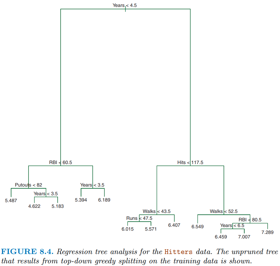

CART uses binary recursive partitioning

Recursive simply means that each split (or rule) depends on the the splits above it:

The algorithm first identifies the “best” feature to partition the observations in the root node into one of two new regions (i.e., new nodes that will be on the left and right branches leading from the root node.)
- For regression problems, the “best” feature (and the rule using that feature) is the feature that maximizes the reduction in SSE
- For classification problems, the split is selected to maximize the reduction in cross-entropy or the Gini index. These are measures of impurity (and we want to get homogeneous nodes so we minimize them)
The splitting process is then repeated on each of the two new nodes (hence the name binary recursive partitioning).
This process is continued until a suitable stopping criterion is reached.

The final depth of the tree is what affects the bias/variance trade-off for this algorithm

Deep trees (with smaller and smaller sized nodes) will have lower and lower bias but can become overfit to the training data
Shallow trees may be overly biased (underfit)

There are two primary approaches to achieve the optimal balance in the bias-variance trade-off

Early stopping
Pruning

With early stopping:

We explicitly stop the growth of the tree early based on a stopping rule. The two most common are:
- A maximum tree depth is reached
- The node has too few cases to be considered for further splits
These two stopping criteria can be implemented independently of each other but they do interact
They should ideally be tuned via the cross-validation approaches we have learned

With pruning, we let the tree grow large (max depth = 30 on 32-bit machines) and then prune it back to an optimal size:

To do this, we apply a penalty (\(\lambda\) * # of terminal nodes) to the cost function/impurity index (analogous to the L1/LASSO penalty). This penalty is also referred to as the cost complexity parameter
Big values for cost complexity will result in less complex trees. Small values will result in deeper, more complex trees
Cost complexity can be tuned by our standard cross-validation approaches by itself or in combination with the previous two hyper parameters

Feature engineering for decision trees can be simpler than with other algorithms because there are very few pre-processing requirements:

Monotonic transformations (e.g., power transformations) are not required to meet algorithm assumptions (in contrast to many parametric models). These transformations only shift the location of the optimal split points.
Outliers typically do not bias the results as much since the binary partitioning simply looks for a single location to make a split within the distribution of each feature.
The algorithm will handle non-linear effects of features and interactions natively
Categorical predictors do not need pre-processing to convert to numeric (e.g., dummy coding).
For unordered categorical features with more than two levels, the classes are ordered based on the outcome
- For regression problems, the mean of the response is used
- For classification problems, the proportion of the positive outcome class is used.
- This means that aggregating response levels is not necessary
Most decision tree implementations (including the rpart engine) can easily handle missing values in the features and do not require imputation. In rpart, this is handled by using surrogate splits.

It is important to note that feature engineering (e.g., alternative strategies for missing data, categorical level aggregation) may still improve performance, but this algorithm does not have the same pre-processing requirements we have seen previously and will work fairly well “out of the box”.

9.3 Decision Trees in Ames

Let’s see this algorithm in action

We will explore the decision tree algorithm (and ensemble approaches using it) with the Ames Housing Prices database
Parallel processing is VERY useful for ensemble approaches because they can be computationally costly

Read the Ames dataset

All predictors
Set factors
Some tidying of variable names and responses

data_trn <- read_csv(here::here(path_data, "ames_raw_class.csv"),
              col_types = cols()) |>   
  janitor::clean_names(case = "snake") |> 
  mutate(exter_qual = replace_na(exter_qual, "none"),
         bsmt_qual = replace_na(bsmt_qual, "none"),
         kitchen_qual = replace_na(kitchen_qual, "none"),
         garage_qual = replace_na(garage_qual, "none"),
         fireplace_qu = replace_na(fireplace_qu, "none"),
         alley = replace_na(alley, "none"),
         bsmt_cond = replace_na(bsmt_cond, "none"),
         bsmt_exposure = replace_na(bsmt_exposure, "none"),
         bsmt_fin_type_1 = replace_na(bsmt_fin_type_1, "none"),
         bsmt_fin_type_2 = replace_na(bsmt_fin_type_2, "none"),
         garage_type = replace_na(garage_type, "none"),
         garage_finish = replace_na(garage_finish, "none"),
         garage_cond = replace_na(garage_cond, "none"),
         pool_qc = replace_na(pool_qc, "none"),
         fence = replace_na(fence, "none"),
         misc_feature = replace_na(misc_feature, "none"))  |> 
  mutate(across(where(is.character), factor)) |> 
  mutate(across(where(is.factor), tidy_responses)) |> 
  mutate(mo_sold = factor(mo_sold, 
                          levels = 1:12,
                          labels = c("jan", "feb", "mar", "apr", "may", "jun",
                                     "jul", "aug", "sep", "oct", "nov", "dec"))) |> 
  mutate(ms_zoning = fct_recode(ms_zoning,
                                res_low = "rl",
                                res_med = "rm",
                                res_high = "rh",
                                float = "fv",
                                agri = "a_agr",
                                indus = "i_all",
                                commer = "c_all"),
         bldg_type = fct_recode(bldg_type,
                                one_fam = "1fam",
                                two_fam = "2fmcon",
                                town_end = "twnhse",
                                town_inside = "twnhs")) |>
  select(-pid)

And take a quick look

data_trn |> skim_some()

Data summary
Name	data_trn
Number of rows	1955
Number of columns	80
_______________________
Column type frequency:
factor	45
numeric	35
________________________
Group variables	None

Variable type: factor

skim_variable	n_missing	complete_rate	ordered	n_unique	top_counts
ms_sub_class	0	1.00	FALSE	16	020: 730, 060: 388, 050: 208, 120: 122
ms_zoning	0	1.00	FALSE	7	res: 1530, res: 297, flo: 91, com: 19
street	0	1.00	FALSE	2	pav: 1946, grv: 9
alley	0	1.00	FALSE	3	non: 1821, grv: 86, pav: 48
lot_shape	0	1.00	FALSE	4	reg: 1258, ir1: 636, ir2: 49, ir3: 12
land_contour	0	1.00	FALSE	4	lvl: 1769, hls: 75, bnk: 72, low: 39
utilities	0	1.00	FALSE	2	all: 1953, nos: 2
lot_config	0	1.00	FALSE	5	ins: 1454, cor: 328, cul: 114, fr2: 55
land_slope	0	1.00	FALSE	3	gtl: 1864, mod: 78, sev: 13
neighborhood	0	1.00	FALSE	28	nam: 299, col: 174, old: 161, edw: 135
condition_1	0	1.00	FALSE	9	nor: 1693, fee: 114, art: 54, rra: 31
condition_2	0	1.00	FALSE	6	nor: 1938, fee: 6, art: 4, pos: 3
bldg_type	0	1.00	FALSE	5	one: 1631, tow: 145, dup: 77, tow: 64
house_style	0	1.00	FALSE	8	1st: 989, 2st: 580, 1_5: 224, slv: 79
roof_style	0	1.00	FALSE	6	gab: 1557, hip: 362, gam: 16, fla: 9
roof_matl	0	1.00	FALSE	7	com: 1929, tar: 11, wds: 8, wds: 4
exterior_1st	0	1.00	FALSE	15	vin: 671, hdb: 301, met: 298, wd_: 283
exterior_2nd	0	1.00	FALSE	17	vin: 662, met: 295, hdb: 279, wd_: 267
mas_vnr_type	17	0.99	FALSE	5	non: 1167, brk: 581, sto: 171, brk: 18
exter_qual	0	1.00	FALSE	4	ta: 1215, gd: 651, ex: 63, fa: 26
exter_cond	0	1.00	FALSE	5	ta: 1707, gd: 195, fa: 42, ex: 8
foundation	0	1.00	FALSE	6	pco: 865, cbl: 849, brk: 198, sla: 33
bsmt_qual	0	1.00	FALSE	5	ta: 861, gd: 808, ex: 167, fa: 62
bsmt_cond	0	1.00	FALSE	6	ta: 1739, gd: 85, fa: 69, non: 57
bsmt_exposure	0	1.00	FALSE	5	no: 1271, av: 274, gd: 183, mn: 168
bsmt_fin_type_1	0	1.00	FALSE	7	unf: 576, glq: 535, alq: 294, rec: 202
bsmt_fin_type_2	0	1.00	FALSE	7	unf: 1655, rec: 75, lwq: 69, non: 57
heating	0	1.00	FALSE	6	gas: 1920, gas: 20, gra: 8, wal: 5
heating_qc	0	1.00	FALSE	5	ex: 979, ta: 590, gd: 324, fa: 60
central_air	0	1.00	FALSE	2	y: 1821, n: 134
electrical	1	1.00	FALSE	5	sbr: 1792, fus: 125, fus: 29, fus: 7
kitchen_qual	0	1.00	FALSE	5	ta: 1011, gd: 765, ex: 126, fa: 52
functional	0	1.00	FALSE	8	typ: 1822, min: 48, min: 41, mod: 23
fireplace_qu	0	1.00	FALSE	6	non: 960, gd: 481, ta: 407, fa: 44
garage_type	0	1.00	FALSE	7	att: 1161, det: 521, bui: 123, non: 107
garage_finish	0	1.00	FALSE	4	unf: 826, rfn: 547, fin: 473, non: 109
garage_qual	0	1.00	FALSE	6	ta: 1745, non: 109, fa: 79, gd: 16
garage_cond	0	1.00	FALSE	6	ta: 1778, non: 109, fa: 46, gd: 12
paved_drive	0	1.00	FALSE	3	y: 1775, n: 139, p: 41
pool_qc	0	1.00	FALSE	5	non: 1945, ex: 3, gd: 3, fa: 2
fence	0	1.00	FALSE	5	non: 1599, mnp: 215, gdw: 70, gdp: 61
misc_feature	0	1.00	FALSE	5	non: 1887, she: 62, oth: 3, gar: 2
mo_sold	0	1.00	FALSE	12	jun: 333, jul: 298, may: 273, apr: 177
sale_type	0	1.00	FALSE	10	wd: 1695, new: 158, cod: 57, con: 16
sale_condition	0	1.00	FALSE	6	nor: 1616, par: 161, abn: 120, fam: 30

Variable type: numeric

skim_variable	n_missing	complete_rate	p0	p100
lot_frontage	319	0.84	21	313
lot_area	0	1.00	1476	215245
overall_qual	0	1.00	1	10
overall_cond	0	1.00	1	9
year_built	0	1.00	1875	2010
year_remod_add	0	1.00	1950	2010
mas_vnr_area	17	0.99	0	1600
bsmt_fin_sf_1	1	1.00	0	5644
bsmt_fin_sf_2	1	1.00	0	1526
bsmt_unf_sf	1	1.00	0	2153
total_bsmt_sf	1	1.00	0	6110
x1st_flr_sf	0	1.00	372	4692
x2nd_flr_sf	0	1.00	0	2065
low_qual_fin_sf	0	1.00	0	1064
gr_liv_area	0	1.00	438	5642
bsmt_full_bath	1	1.00	0	3
bsmt_half_bath	1	1.00	0	2
full_bath	0	1.00	0	4
half_bath	0	1.00	0	2
bedroom_abv_gr	0	1.00	0	8
kitchen_abv_gr	0	1.00	0	3
tot_rms_abv_grd	0	1.00	3	14
fireplaces	0	1.00	0	3
garage_yr_blt	109	0.94	1896	2010
garage_cars	1	1.00	0	4
garage_area	1	1.00	0	1488
wood_deck_sf	0	1.00	0	870
open_porch_sf	0	1.00	0	742
enclosed_porch	0	1.00	0	552
x3ssn_porch	0	1.00	0	508
screen_porch	0	1.00	0	576
pool_area	0	1.00	0	738
misc_val	0	1.00	0	12500
yr_sold	0	1.00	2006	2010
sale_price	0	1.00	12789	745000

A basic recipe for Decision Tree approaches

Easy to do because the algorithm is very flexible
Will handle non-linear relationships and interactions natively
Dummy coding not needed (and generally not recommended) for factors
Not even very important to consider frequency of response categories
Not even necessary to convert character to factor (but I do to make it easy to do further feature engineering if desired)
Be careful with categorical variables which are coded with numbers
- They will be coded as numeric by R and treated as numeric by R
- If they are ordered (overall_qual), this a priori order would be respected by rpart so no worries
- If they are unordered, this will force an order on the levels rather than allowing rpart to determine an order based on the outcome in your training data.
Notice the missing data for features (rpart will handle it with surrogates)

rec <- recipe(sale_price ~ ., data = data_trn)
 
rec_prep <- rec |> 
  prep(data_trn)

feat_trn <- rec_prep |> 
  bake(NULL)

feat_trn |> skim_some()

Data summary
Name	feat_trn
Number of rows	1955
Number of columns	80
_______________________
Column type frequency:
factor	45
numeric	35
________________________
Group variables	None

Variable type: factor

skim_variable	n_missing	complete_rate	ordered	n_unique	top_counts
ms_sub_class	0	1.00	FALSE	16	020: 730, 060: 388, 050: 208, 120: 122
ms_zoning	0	1.00	FALSE	7	res: 1530, res: 297, flo: 91, com: 19
street	0	1.00	FALSE	2	pav: 1946, grv: 9
alley	0	1.00	FALSE	3	non: 1821, grv: 86, pav: 48
lot_shape	0	1.00	FALSE	4	reg: 1258, ir1: 636, ir2: 49, ir3: 12
land_contour	0	1.00	FALSE	4	lvl: 1769, hls: 75, bnk: 72, low: 39
utilities	0	1.00	FALSE	2	all: 1953, nos: 2
lot_config	0	1.00	FALSE	5	ins: 1454, cor: 328, cul: 114, fr2: 55
land_slope	0	1.00	FALSE	3	gtl: 1864, mod: 78, sev: 13
neighborhood	0	1.00	FALSE	28	nam: 299, col: 174, old: 161, edw: 135
condition_1	0	1.00	FALSE	9	nor: 1693, fee: 114, art: 54, rra: 31
condition_2	0	1.00	FALSE	6	nor: 1938, fee: 6, art: 4, pos: 3
bldg_type	0	1.00	FALSE	5	one: 1631, tow: 145, dup: 77, tow: 64
house_style	0	1.00	FALSE	8	1st: 989, 2st: 580, 1_5: 224, slv: 79
roof_style	0	1.00	FALSE	6	gab: 1557, hip: 362, gam: 16, fla: 9
roof_matl	0	1.00	FALSE	7	com: 1929, tar: 11, wds: 8, wds: 4
exterior_1st	0	1.00	FALSE	15	vin: 671, hdb: 301, met: 298, wd_: 283
exterior_2nd	0	1.00	FALSE	17	vin: 662, met: 295, hdb: 279, wd_: 267
mas_vnr_type	17	0.99	FALSE	5	non: 1167, brk: 581, sto: 171, brk: 18
exter_qual	0	1.00	FALSE	4	ta: 1215, gd: 651, ex: 63, fa: 26
exter_cond	0	1.00	FALSE	5	ta: 1707, gd: 195, fa: 42, ex: 8
foundation	0	1.00	FALSE	6	pco: 865, cbl: 849, brk: 198, sla: 33
bsmt_qual	0	1.00	FALSE	5	ta: 861, gd: 808, ex: 167, fa: 62
bsmt_cond	0	1.00	FALSE	6	ta: 1739, gd: 85, fa: 69, non: 57
bsmt_exposure	0	1.00	FALSE	5	no: 1271, av: 274, gd: 183, mn: 168
bsmt_fin_type_1	0	1.00	FALSE	7	unf: 576, glq: 535, alq: 294, rec: 202
bsmt_fin_type_2	0	1.00	FALSE	7	unf: 1655, rec: 75, lwq: 69, non: 57
heating	0	1.00	FALSE	6	gas: 1920, gas: 20, gra: 8, wal: 5
heating_qc	0	1.00	FALSE	5	ex: 979, ta: 590, gd: 324, fa: 60
central_air	0	1.00	FALSE	2	y: 1821, n: 134
electrical	1	1.00	FALSE	5	sbr: 1792, fus: 125, fus: 29, fus: 7
kitchen_qual	0	1.00	FALSE	5	ta: 1011, gd: 765, ex: 126, fa: 52
functional	0	1.00	FALSE	8	typ: 1822, min: 48, min: 41, mod: 23
fireplace_qu	0	1.00	FALSE	6	non: 960, gd: 481, ta: 407, fa: 44
garage_type	0	1.00	FALSE	7	att: 1161, det: 521, bui: 123, non: 107
garage_finish	0	1.00	FALSE	4	unf: 826, rfn: 547, fin: 473, non: 109
garage_qual	0	1.00	FALSE	6	ta: 1745, non: 109, fa: 79, gd: 16
garage_cond	0	1.00	FALSE	6	ta: 1778, non: 109, fa: 46, gd: 12
paved_drive	0	1.00	FALSE	3	y: 1775, n: 139, p: 41
pool_qc	0	1.00	FALSE	5	non: 1945, ex: 3, gd: 3, fa: 2
fence	0	1.00	FALSE	5	non: 1599, mnp: 215, gdw: 70, gdp: 61
misc_feature	0	1.00	FALSE	5	non: 1887, she: 62, oth: 3, gar: 2
mo_sold	0	1.00	FALSE	12	jun: 333, jul: 298, may: 273, apr: 177
sale_type	0	1.00	FALSE	10	wd: 1695, new: 158, cod: 57, con: 16
sale_condition	0	1.00	FALSE	6	nor: 1616, par: 161, abn: 120, fam: 30

Variable type: numeric

skim_variable	n_missing	complete_rate	p0	p100
lot_frontage	319	0.84	21	313
lot_area	0	1.00	1476	215245
overall_qual	0	1.00	1	10
overall_cond	0	1.00	1	9
year_built	0	1.00	1875	2010
year_remod_add	0	1.00	1950	2010
mas_vnr_area	17	0.99	0	1600
bsmt_fin_sf_1	1	1.00	0	5644
bsmt_fin_sf_2	1	1.00	0	1526
bsmt_unf_sf	1	1.00	0	2153
total_bsmt_sf	1	1.00	0	6110
x1st_flr_sf	0	1.00	372	4692
x2nd_flr_sf	0	1.00	0	2065
low_qual_fin_sf	0	1.00	0	1064
gr_liv_area	0	1.00	438	5642
bsmt_full_bath	1	1.00	0	3
bsmt_half_bath	1	1.00	0	2
full_bath	0	1.00	0	4
half_bath	0	1.00	0	2
bedroom_abv_gr	0	1.00	0	8
kitchen_abv_gr	0	1.00	0	3
tot_rms_abv_grd	0	1.00	3	14
fireplaces	0	1.00	0	3
garage_yr_blt	109	0.94	1896	2010
garage_cars	1	1.00	0	4
garage_area	1	1.00	0	1488
wood_deck_sf	0	1.00	0	870
open_porch_sf	0	1.00	0	742
enclosed_porch	0	1.00	0	552
x3ssn_porch	0	1.00	0	508
screen_porch	0	1.00	0	576
pool_area	0	1.00	0	738
misc_val	0	1.00	0	12500
yr_sold	0	1.00	2006	2010
sale_price	0	1.00	12789	745000

Fit a simple decision tree

Use rpart engine
tree_depth = 3
min_n = 2 and cost_complexity = 0 removes impact of those hyperparameters
model = TRUE if you want to plot the decision tree with rplot.plot() from the rpart.plot package

fit_tree_ex1 <-   
  decision_tree(tree_depth = 3, min_n = 2, cost_complexity = 0) |>
  set_engine("rpart", model = TRUE) |>
  set_mode("regression") |>  
  fit(sale_price ~ garage_cars + garage_area + overall_qual + kitchen_qual +
                  bsmt_qual, data = feat_trn)

Let’s plot the decision tree using rpart.plot for a package with the same name. No need to load the full package

Easy to understand how the model makes predictions

fit_tree_ex1$fit |> rpart.plot::rpart.plot()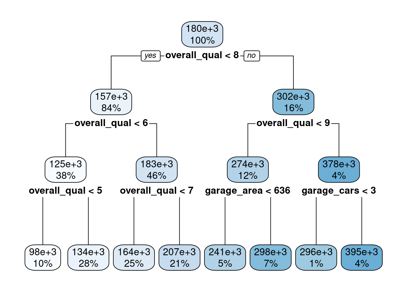

Question: How can we determine how well this model predicts sale_price?

Show Answer

We need held out data. We could do a validation split, k-fold, or bootstraps.  
K-fold may be preferred b/c it provides a less biased estimate of model performance.  
I will use bootstrap cross-validation instead because I will later use these same 
splits to also choose among hyperparameter values.]

Using only 10 bootstraps to save time. Use more in your work!

set.seed(20140102)
splits_boot <- data_trn |> 
  bootstraps(times = 10, strata = "sale_price")

Now let’s evaluate its performance in our OOB held-out sets

fits_tree_ex1 <- cache_rds(
  expr = {
  decision_tree(tree_depth = 3, min_n = 2, cost_complexity = 0) |>
    set_engine("rpart") |>
    set_mode("regression") |> 
    fit_resamples(preprocessor = rec, 
              resamples = splits_boot,  
              metrics = metric_set(rmse))
  },
  rerun = rerun_setting,
  dir = "cache/009/",
  file = "fits_tree_ex1")

Not that great (remember unit 3 with only a subset of predictors did better than this)

fits_tree_ex1 |> collect_metrics()

# A tibble: 1 × 6
  .metric .estimator   mean     n std_err .config             
  <chr>   <chr>       <dbl> <int>   <dbl> <chr>               
1 rmse    standard   42771.   100    271. Preprocessor1_Model1

We want to allow a deeper tree to reduce bias

But will also need to consider pruning tree to prevent overfitting

This is the bias-variance trade-off again. To find the sweet stop we can tune

tree_depth
min_n
cost_complexity

Set up a tuning grid

Can use tidymodels to determine possibly good values to start
Still need to evaluate
May still need to adjust

cost_complexity()

Cost-Complexity Parameter (quantitative)
Transformer: log-10 [1e-100, Inf]
Range (transformed scale): [-10, -1]

tree_depth()

Tree Depth (quantitative)
Range: [1, 15]

min_n()

Minimal Node Size (quantitative)
Range: [2, 40]

We can use these function with dials::grid_regular() to get a tuning grid

With levels = 4 we get 64 combinations of values (4 x 4 x 4)

grid_tree <- grid_regular(cost_complexity(), tree_depth(), min_n(), levels = 4)

grid_tree

# A tibble: 64 × 3
   cost_complexity tree_depth min_n
             <dbl>      <int> <int>
 1    0.0000000001          1     2
 2    0.0000001             1     2
 3    0.0001                1     2
 4    0.1                   1     2
 5    0.0000000001          5     2
 6    0.0000001             5     2
 7    0.0001                5     2
 8    0.1                   5     2
 9    0.0000000001         10     2
10    0.0000001            10     2
# ℹ 54 more rows

Now we can use the bootstrap as intended to select best values of hyperparameters (i.e., tune them)

fits_tree <- cache_rds(
  expr = {
    decision_tree(cost_complexity = tune(),
                tree_depth = tune(),
                min_n = tune()) |>
    set_engine("rpart") |>
    set_mode("regression") |> 
    tune_grid(preprocessor = rec, 
              resamples = splits_boot, 
              grid = grid_tree, 
              metrics = metric_set(rmse))

  },
  rerun = rerun_setting,
  dir = "cache/009",
  file = "fits_tree")

Can use autoplot() to view performance by hyperparameter values

# autoplot(fits_tree)

The best values for some of the hyperparameters (tree depth and min n) are at their edges so we might consider extending their range and training again. I will skip this here to save time.

This model as good as our other models in unit 3 (see OOB cross-validated error above). It was easy to fit with all the predictors. It might get even a little better for we further tuned the hyperparameters. However, we can still do better with a more advanced algorithm based on decision trees.

show_best(fits_tree)

# A tibble: 5 × 9
  cost_complexity tree_depth min_n .metric .estimator   mean     n std_err
            <dbl>      <int> <int> <chr>   <chr>       <dbl> <int>   <dbl>
1    0.0001               15    40 rmse    standard   37151.   100    219.
2    0.0000000001         10    40 rmse    standard   37154.   100    220.
3    0.0000001            10    40 rmse    standard   37154.   100    220.
4    0.0000000001         15    40 rmse    standard   37154.   100    219.
5    0.0000001            15    40 rmse    standard   37154.   100    219.
  .config              
  <chr>                
1 Preprocessor1_Model63
2 Preprocessor1_Model57
3 Preprocessor1_Model58
4 Preprocessor1_Model61
5 Preprocessor1_Model62

Let’s still fit this tree to all the training data and understand it a bit better

fit_tree <-   
  decision_tree(cost_complexity = select_best(fits_tree)$cost_complexity,
                tree_depth = select_best(fits_tree)$tree_depth,
                min_n = select_best(fits_tree)$min_n) |>
  set_engine("rpart", model = TRUE) |>
  set_mode("regression") |>  
  fit(sale_price ~ ., data = feat_trn)

Still interpretable but need bigger, higher res plot

fit_tree$fit |> rpart.plot::rpart.plot()

Warning: labs do not fit even at cex 0.15, there may be some overplotting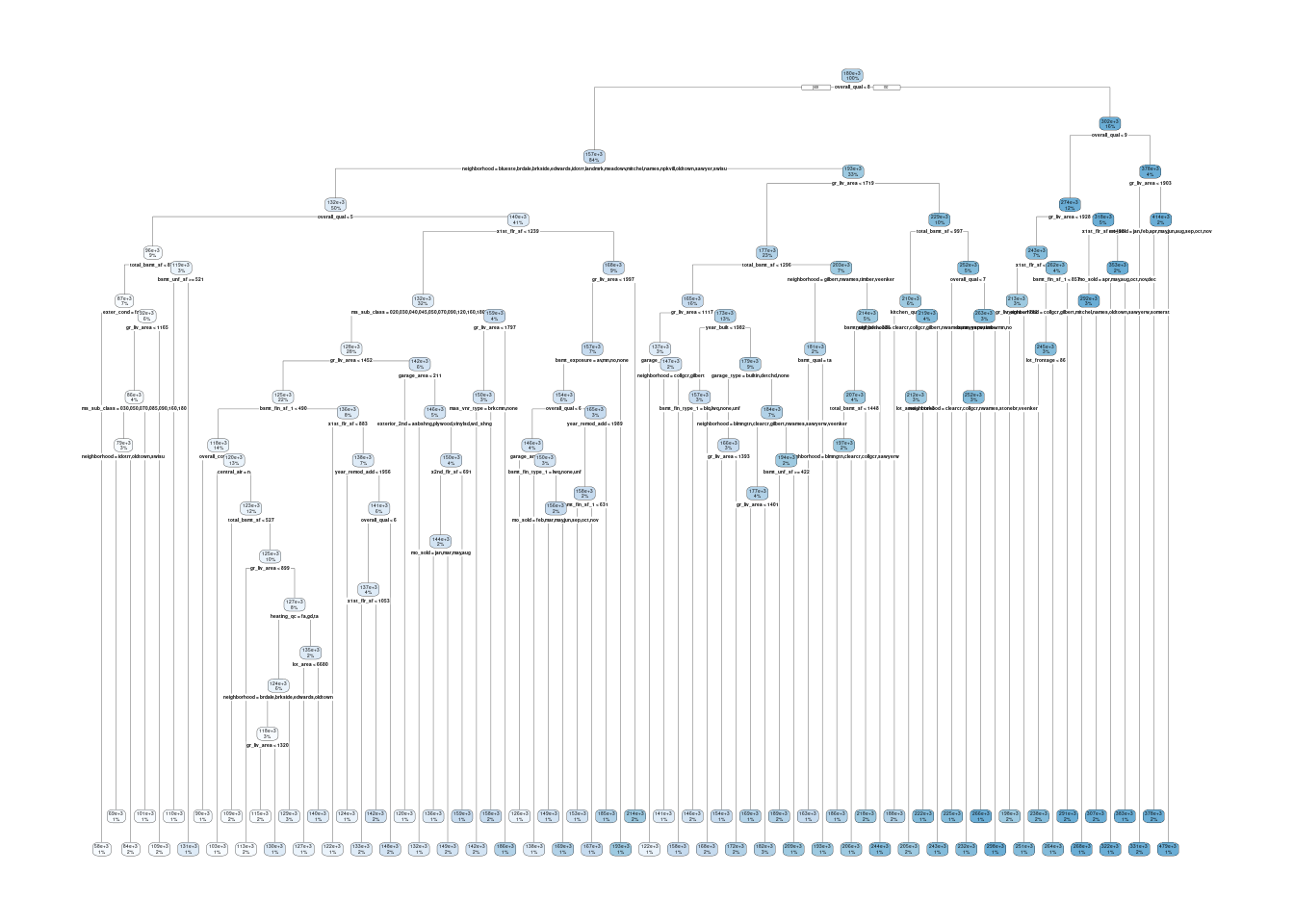

Even though decision trees themselves are relatively poor at prediction, these ideas will be key when we consider more advanced ensemble approaches

Ensemble approaches aggregate multiple models to improve prediction. Our first ensemble approach is bagging.

9.4 Bagging

Bootstrap aggregating (bagging) prediction models involve:

Fitting multiple versions of a prediction model
Combining (or ensembling) them into an aggregated prediction
You can begin to learn more about bagging in the original paper that proposed the technique

The specific steps are:

B bootstraps of the original training data are created [NOTE: This is a new use for bootstrapping! More on that in a moment]
The model configuration (either regression or classification algorithm with a specific set of features and hyperparameters) is fit to each bootstrap sample
These individual fitted models are called the base learners
Final predictions are made by aggregating the predictions across all of the individual base learners
- For regression, this can be the average of base learner predictions
- For classification, it can be either the average of estimated class probabilities or majority class vote across individual base learners

Bagging effectively reduces the variance of an individual base learner

However, bagging does not always improve on an individual base learner

Bagging works especially well for flexible, high variance base learners (based on statistical algorithms or other characteristics of the problem)
These base learners can become overfit to their training data
Therefore base learners will produce different predictions across each bootstrap sample of the training data
The aggregate predictions across base learners will be lower variance
With respect to statistical algorithms that you know, decision trees are high variance (KNN also)
In contrast, bagging a linear model (with low P to N ratio) would likely not improve much upon the base learners’ performance

Bagging takes advantage of the “wisdom of the crowd” effect (Surowiecki, 2005)

Aggregation of information across large diverse groups often produces decisions that are better than any single member of the group
Regis Philbin once stated that the Ask the Audience lifeline on Who Wants to be a Millionaire is right 95% of the time
With more diverse group members and perspectives (i.e., high variance learners), we get better aggregated predictions

With decision trees, optimal performance is often found by bagging 50-500 base learner trees

Data sets that have a few strong features typically require fewer trees
Data sets with lots of noise or multiple strong features may need more
Using too many trees will NOT lead to overfitting, just no further benefit in variance reduction
However, too many trees will increase computational costs (particularly if you are also using “an outer loop” of resampling to select among configurations or to evaluate the model)

Bagging uses bootstrap resampling for yet another goal. We can use bootstrapping

For cross-validation to assess performance model configuration(s)
- Select among model model configurations
- Evaluate a final model configuration (if we don’t have independent test set)
For estimating standard errors and confidence intervals of statistics (no longer part of this course - see Appendix)
And now for building multiple base learners whose aggregate predictions are lower variance than any of the individual base learners

When bagging, we can (and typically will):

Use an “outer loop” of bootstrap resampling to select among model configurations
While using an “inner loop” of bootstrapping to fit multiple base learners for any specific configuration
This inner loop is often opaque to users (more on this in a moment), happening under the hood in the algorithm (e.g., Random Forest) or the implementation of the code (bagged_tree())

9.5 Bagging Trees in Ames

We will now use bag_tree() rather than decision_tree() from the baguette package. Not part of minimal tidymodels libraries so we will need to load this package

library(baguette)

We can still tune the same hyperparameters. We are now just creating many rpart decision trees and aggregating their predictions. We will START with the recommended values by tidymodels

We can use the same recipe

We will use the same splits to tune hyperparameters

Now we need times = 20 to fit 20 models (inner loop of bootstrapping) to each of the 10 bootstraps (outer loop; set earlier) of the training data.

Keeping this low to reduce computational costs.
You will likely want more bootstrapped models to reduce final model variance and more boostraps resamples to get a lower variance performance estimate to select best hyperparameters

fits_bagged <- cache_rds(
  expr = {
    bag_tree(cost_complexity = tune(),
           tree_depth = tune(),
           min_n = tune()) |>
    set_engine("rpart", times = 20) |>
    set_mode("regression") |> 
    tune_grid(preprocessor = rec, 
              resamples = splits_boot, 
              grid = grid_tree, 
              metrics = metric_set(rmse))

  },
  rerun = rerun_setting,
  dir = "cache/009/",
  file = "fits_bagged")

Can still use autoplot() to view performance by hyperparameter values

# autoplot(fits_bagged)

The best values for all hyperparameters are at their edges.

Looks like we could have fit a more complex model.
Makes sense because we are relying on bagging to reduce model variance so we can accommodate base learners that are more overfit.

show_best(fits_bagged)

# A tibble: 5 × 9
  cost_complexity tree_depth min_n .metric .estimator   mean     n std_err
            <dbl>      <int> <int> <chr>   <chr>       <dbl> <int>   <dbl>
1    0.0000001            15     2 rmse    standard   27777.    10    537.
2    0.0001               15     2 rmse    standard   27801.    10    644.
3    0.0001               15    14 rmse    standard   27870.    10    748.
4    0.0000000001         10    14 rmse    standard   27908.    10    777.
5    0.0000000001         10     2 rmse    standard   27910.    10    609.
  .config              
  <chr>                
1 Preprocessor1_Model14
2 Preprocessor1_Model15
3 Preprocessor1_Model31
4 Preprocessor1_Model25
5 Preprocessor1_Model09

Switching to expand_grid() to manually select

grid_tree_bagged <- expand_grid(cost_complexity = c(10^-10, 10^-7, 10^-04, 10^-01), 
                                tree_depth = c(10, 15, 20, 30), 
                                min_n = c(2, 14, 27, 40))

grid_tree_bagged

# A tibble: 64 × 3
   cost_complexity tree_depth min_n
             <dbl>      <dbl> <dbl>
 1    0.0000000001         10     2
 2    0.0000000001         10    14
 3    0.0000000001         10    27
 4    0.0000000001         10    40
 5    0.0000000001         15     2
 6    0.0000000001         15    14
 7    0.0000000001         15    27
 8    0.0000000001         15    40
 9    0.0000000001         20     2
10    0.0000000001         20    14
# ℹ 54 more rows

fits_bagged_2 <- cache_rds(
  expr = {
    bag_tree(cost_complexity = tune(),
           tree_depth = tune(),
           min_n = tune()) |>
    set_engine("rpart", times = 20) |>
    set_mode("regression") |> 
    tune_grid(preprocessor = rec, 
              resamples = splits_boot, 
              grid = grid_tree_bagged, 
              metrics = metric_set(rmse))
  },
  rerun = rerun_setting, 
  dir = "cache/009/",
  file = "fits_bagged_2")

Review hyperparameter plot

# autoplot(fits_bagged_2)

This looks better. And look at that BIG improvement in OOB cross-validated RMSE

show_best(fits_bagged_2)

# A tibble: 5 × 9
  cost_complexity tree_depth min_n .metric .estimator   mean     n std_err
            <dbl>      <dbl> <dbl> <chr>   <chr>       <dbl> <int>   <dbl>
1    0.0001               15     2 rmse    standard   27575.    10    640.
2    0.0000000001         15     2 rmse    standard   27673.    10    635.
3    0.0000001            30     2 rmse    standard   27724.    10    662.
4    0.0000001            20     2 rmse    standard   27726.    10    713.
5    0.0000000001         20     2 rmse    standard   27758.    10    625.
  .config              
  <chr>                
1 Preprocessor1_Model37
2 Preprocessor1_Model05
3 Preprocessor1_Model29
4 Preprocessor1_Model25
5 Preprocessor1_Model09

BUT, we can do better still…..

9.6 Random Forest

Random forests are a modification of bagged decision trees that build a large collection of de-correlated trees to further improve predictive performance.

They are a very popular “out-of-the-box” or “off-the-shelf” statistical algorithm that predicts well
Many modern implementations of random forests exist; however, Breiman’s algorithm (Breiman 2001) has largely become the standard procedure.
We will use the ranger engine implementation of this algorithm

Random forests build on decision trees (its base learners) and bagging to reduce final model variance.

Simply bagging trees is not optimal to reduce final model variance

The trees in bagging are not completely independent of each other since all the original features are considered at every split of every tree.
Trees from different bootstrap samples typically have similar structure to each other (especially at the top of the tree) due to any underlying strong relationships
The trees are correlated (not as diverse a set of base learners)

Random forests help to reduce tree correlation by injecting more randomness into the tree-growing process

More specifically, while growing a decision tree during the bagging process, random forests perform split-variable randomization where each time a split is to be performed, the search for the best split variable is limited to a random subset of mtry of the original p features.

Because the algorithm randomly selects a bootstrap sample to train on and a random sample of features to use at each split, a more diverse set of trees is produced which tends to lessen tree correlation beyond bagged trees and often dramatically increases predictive power.

There are three primary hyper-parameters to consider tuning in random forests within tidymodels

mtry
trees
min_n

mtry

The number of features to randomly select for splitting on each split
Selection of value for mtry balances low tree correlation with reasonable predictive strength
Good starting values for mtry are \(\frac{p}{3}\) for regression and \(\sqrt{p}\) for classification
When there are fewer relevant features (e.g., noisy data) a higher value may be needed to make it more likely to select those features with the strongest signal.
When there are many relevant features, a lower value might perform better
Default in ranger is \(\sqrt{p}\)

trees

The number of bootstrap resamples of the training data to fit decision tree base learners
The number of trees needs to be sufficiently large to stabilize the error rate.
A good rule of thumb is to start with 10 times the number of features
You may need to adjust based on values for mtry and min_n
More trees provide more robust and stable error estimates and variable importance measures
More trees == more computational cost
Default in ranger is 500

min_n

Minimum number of observations in a new node rather than min to split
Note that this is different than its definition for decision trees and bagged trees
You can consider the defaults (above) as a starting point
If your data has many noisy predictors and higher mtry values are performing best, then performance may improve by increasing node size (i.e., decreasing tree depth and complexity).
If computation time is a concern then you can often decrease run time substantially by increasing the node size and have only marginal impacts to your error estimate
Default in ranger is 1 for classification and 5 for regression

9.6.1 Random Forest in Ames

Let’s see how de-correlated the base learner trees improves their aggregate performance

We will need a new recipe for Random Forest

Random Forest works well out of the box with little feature engineering
It is still aggregating decision trees in bootstrap resamples of the training data
However, the Random Forest algorithm does not natively handling missing data. We need to handle missing data manually during feature engineering. We will impute

rec_rf <- recipe(sale_price ~ ., data = data_trn) |> 
  step_impute_median(all_numeric()) |> 
  step_impute_mode(all_nominal()) 

rec_rf_prep <- rec_rf |>
  prep(data_trn)

feat_trn_rf <- rec_rf_prep |> 
  bake(NULL)

A quick look at features

feat_trn_rf |> skim_some()

Data summary
Name	feat_trn_rf
Number of rows	1955
Number of columns	80
_______________________
Column type frequency:
factor	45
numeric	35
________________________
Group variables	None

Variable type: factor

skim_variable	complete_rate	ordered	n_unique	top_counts
ms_sub_class	1	FALSE	16	020: 730, 060: 388, 050: 208, 120: 122
ms_zoning	1	FALSE	7	res: 1530, res: 297, flo: 91, com: 19
street	1	FALSE	2	pav: 1946, grv: 9
alley	1	FALSE	3	non: 1821, grv: 86, pav: 48
lot_shape	1	FALSE	4	reg: 1258, ir1: 636, ir2: 49, ir3: 12
land_contour	1	FALSE	4	lvl: 1769, hls: 75, bnk: 72, low: 39
utilities	1	FALSE	2	all: 1953, nos: 2
lot_config	1	FALSE	5	ins: 1454, cor: 328, cul: 114, fr2: 55
land_slope	1	FALSE	3	gtl: 1864, mod: 78, sev: 13
neighborhood	1	FALSE	28	nam: 299, col: 174, old: 161, edw: 135
condition_1	1	FALSE	9	nor: 1693, fee: 114, art: 54, rra: 31
condition_2	1	FALSE	6	nor: 1938, fee: 6, art: 4, pos: 3
bldg_type	1	FALSE	5	one: 1631, tow: 145, dup: 77, tow: 64
house_style	1	FALSE	8	1st: 989, 2st: 580, 1_5: 224, slv: 79
roof_style	1	FALSE	6	gab: 1557, hip: 362, gam: 16, fla: 9
roof_matl	1	FALSE	7	com: 1929, tar: 11, wds: 8, wds: 4
exterior_1st	1	FALSE	15	vin: 671, hdb: 301, met: 298, wd_: 283
exterior_2nd	1	FALSE	17	vin: 662, met: 295, hdb: 279, wd_: 267
mas_vnr_type	1	FALSE	5	non: 1184, brk: 581, sto: 171, brk: 18
exter_qual	1	FALSE	4	ta: 1215, gd: 651, ex: 63, fa: 26
exter_cond	1	FALSE	5	ta: 1707, gd: 195, fa: 42, ex: 8
foundation	1	FALSE	6	pco: 865, cbl: 849, brk: 198, sla: 33
bsmt_qual	1	FALSE	5	ta: 861, gd: 808, ex: 167, fa: 62
bsmt_cond	1	FALSE	6	ta: 1739, gd: 85, fa: 69, non: 57
bsmt_exposure	1	FALSE	5	no: 1271, av: 274, gd: 183, mn: 168
bsmt_fin_type_1	1	FALSE	7	unf: 576, glq: 535, alq: 294, rec: 202
bsmt_fin_type_2	1	FALSE	7	unf: 1655, rec: 75, lwq: 69, non: 57
heating	1	FALSE	6	gas: 1920, gas: 20, gra: 8, wal: 5
heating_qc	1	FALSE	5	ex: 979, ta: 590, gd: 324, fa: 60
central_air	1	FALSE	2	y: 1821, n: 134
electrical	1	FALSE	5	sbr: 1793, fus: 125, fus: 29, fus: 7
kitchen_qual	1	FALSE	5	ta: 1011, gd: 765, ex: 126, fa: 52
functional	1	FALSE	8	typ: 1822, min: 48, min: 41, mod: 23
fireplace_qu	1	FALSE	6	non: 960, gd: 481, ta: 407, fa: 44
garage_type	1	FALSE	7	att: 1161, det: 521, bui: 123, non: 107
garage_finish	1	FALSE	4	unf: 826, rfn: 547, fin: 473, non: 109
garage_qual	1	FALSE	6	ta: 1745, non: 109, fa: 79, gd: 16
garage_cond	1	FALSE	6	ta: 1778, non: 109, fa: 46, gd: 12
paved_drive	1	FALSE	3	y: 1775, n: 139, p: 41
pool_qc	1	FALSE	5	non: 1945, ex: 3, gd: 3, fa: 2
fence	1	FALSE	5	non: 1599, mnp: 215, gdw: 70, gdp: 61
misc_feature	1	FALSE	5	non: 1887, she: 62, oth: 3, gar: 2
mo_sold	1	FALSE	12	jun: 333, jul: 298, may: 273, apr: 177
sale_type	1	FALSE	10	wd: 1695, new: 158, cod: 57, con: 16
sale_condition	1	FALSE	6	nor: 1616, par: 161, abn: 120, fam: 30

Variable type: numeric

skim_variable	complete_rate	p0	p100
lot_frontage	1	21	313
lot_area	1	1476	215245
overall_qual	1	1	10
overall_cond	1	1	9
year_built	1	1875	2010
year_remod_add	1	1950	2010
mas_vnr_area	1	0	1600
bsmt_fin_sf_1	1	0	5644
bsmt_fin_sf_2	1	0	1526
bsmt_unf_sf	1	0	2153
total_bsmt_sf	1	0	6110
x1st_flr_sf	1	372	4692
x2nd_flr_sf	1	0	2065
low_qual_fin_sf	1	0	1064
gr_liv_area	1	438	5642
bsmt_full_bath	1	0	3
bsmt_half_bath	1	0	2
full_bath	1	0	4
half_bath	1	0	2
bedroom_abv_gr	1	0	8
kitchen_abv_gr	1	0	3
tot_rms_abv_grd	1	3	14
fireplaces	1	0	3
garage_yr_blt	1	1896	2010
garage_cars	1	0	4
garage_area	1	0	1488
wood_deck_sf	1	0	870
open_porch_sf	1	0	742
enclosed_porch	1	0	552
x3ssn_porch	1	0	508
screen_porch	1	0	576
pool_area	1	0	738
misc_val	1	0	12500
yr_sold	1	2006	2010
sale_price	1	12789	745000

We will need a tuning grid for the hyperparameters

I played around a bit with values for trees, mtry, and min_n until I arrived at values that produced a floor for RMSE

grid_rf <- expand_grid(trees = c(250, 500, 750, 1000), 
                       mtry = c(5, 10, 20, 25), 
                       min_n = c(1, 2, 5, 10))

Let’s now fit the model configurations defined by the grid_rf using tune_grid()

ranger gives you a lot of additional control by changing defaults in set_engine().

We will mostly use defaults
You should explore if you want to get the best performance from your models
see ?ranger
Defaults for splitting rules are gini for classification and variance for regression. These are appropriate
We will explicitly specify respect.unordered.factors = "order" as recommended. Could consider respect.unordered.factors = "partition"
We will set oob.error = FALSE. TRUE would allow for OOB performance estimate using OOB for each bootstrap for each base learner. We calculate this ourselves using tune_grid()
We will set seed = to generate reproducible bootstraps

fits_rf <-cache_rds(
  expr = {
    rand_forest(trees = tune(),
              mtry = tune(),
              min_n = tune()) |>
    set_engine("ranger",
               respect.unordered.factors = "order",
               oob.error = FALSE,
               seed = 102030) |>
    set_mode("regression") |> 
    tune_grid(preprocessor = rec_rf, 
              resamples = splits_boot, 
              grid = grid_rf, 
              metrics = metric_set(rmse))

  },
  rerun = rerun_setting,
  dir = "cache/009/",
  file = "fits_rf")

We used these plots to confirm that we had selected good combinations of hyperparameters to tune and that the best hyperparameters are inside the range of values considered (or at their objective edge)

# autoplot(fits_rf)

But more importantly, look at the additional reduction in OOB RMSE for Random Forest relative to bagged trees!

show_best(fits_rf)

# A tibble: 5 × 9
   mtry trees min_n .metric .estimator   mean     n std_err
  <dbl> <dbl> <dbl> <chr>   <chr>       <dbl> <int>   <dbl>
1    20   750     1 rmse    standard   24979.    10    710.
2    20   750     2 rmse    standard   24980.    10    711.
3    20  1000     1 rmse    standard   24981.    10    713.
4    20  1000     2 rmse    standard   24991.    10    716.
5    20   500     1 rmse    standard   24997.    10    717.
  .config              
  <chr>                
1 Preprocessor1_Model41
2 Preprocessor1_Model42
3 Preprocessor1_Model57
4 Preprocessor1_Model58
5 Preprocessor1_Model25

Let’s fit the best model configuration to all the training data

We will use the same seed and other arguments as before
We could now use this final model to predict into our Ames test set (but we will skip that step) to get a better estimate of true performance with new data.

fit_rf <-   
  rand_forest(trees = select_best(fits_rf)$trees,
                mtry = select_best(fits_rf)$mtry,
                min_n = select_best(fits_rf)$min_n) |>
  set_engine("ranger", 
             respect.unordered.factors = "order", 
             oob.error = FALSE,
             seed = 102030) |>
  set_mode("regression") |>  
  fit(sale_price ~ ., data = feat_trn_rf)

In conclusion:

Random Forest is a great out of the box statistical algorithm for both classification and regression
We see no compelling reason to use bagged trees because Random Forest has all (except missing data handling) the benefits of bagged trees plus better prediction b/c of the de-correlated base learners
In some instances, we might use a decision tree if we wanted an interpretable tree as a method to understand rule based relationships between our features and our outcome.

9.7 Discussion Notes

9.7.1 Announcements

Exam answer review
Exam grading questions
Quiz performance and updates (alpha, what would you NEVER do)
Installing keras package

9.7.2 Trees

When we split the data in a tree by a variable, how the threshold is specified? Is the algorithm determining it internally? (It looks like so, but I wonder if we could/should/might decide threshold manully sometime?) How it automatically decides the thresholds: is the tree calculating the accuracy(or other metrics) value at each node for each possible threshold decided by each variable?
Can you explain more on gini and entropy? What are the costs and benefits of them, and how can we determine which to use?
Why isn’t feature engineering required as extensively when it comes to decision trees?
- out of box statistical algorithmsi
How does CART and RF handle categorical variables? What about other transformations of predictors (normalize, scale, combine)? non-linear?
What determines the depth of trees that we set in decision trees and random forest?
Can we compare the advantages or situations when we should choose trees and random forests?
How do trees handle missing data? Do we ever want to impute missing data in our recipes?
Can you give more examples of how to interpret the decision tree graph?

9.7.3 Bagging

When and Why does bagging improve model performance
By bagging the decision trees, what are we trading off for less variance? Is our model more biased in some way? Or are we sacrificing the accuracy of where trees splits for less model variance?
- other examples when we don’t trade off bias/variance of some estimate (one for models, one for performance estimates?)
Can you explain more on why we should de-correlate the bagged trees? Do we not need to de-correlate if we are not using bagging?

9.7.4 Random Forest

I think it would be useful to go over how the hyperparameter values for random forests were chosen in the web book example. Specifically, I don’t understand how the range of values was determined and how I can do this on my own.
When we tune mtry in random forest, how can we determine the best range to tune on? Do we need to find p/3 or p^(1/2) and use that as a midpoint and test a range by hand? Is there no default range for mtry?
When tuning grid for hyperparameters, is there sort of an “intuitive” way to select the values for trees, mtry and min_n?

9.7.5 Boosting

I don’t understand the boosting process very well, especially mathematically, I don’t understand how to “change the outcome of the subsequent trees as the residual of the original tree”. And is the residual here referring the residual of the latest tree? (Because in regression model we want to predict the value and in classification model we try to figure out what the predictors point to, and residual as an outcome is somehow seemingly not included in these two types?) Could we go through boosting tree and Bayesian tree method quickly?

9.7.6 Relative Costs/Benefits of Algorithms

Can we compare the advantages or situations when we should choose trees and random forests?
For which types of data or questions is it best to use boosting vs. regular bagging?
Discuss the advantages and limitations of decision trees compared to other machine learning algorithms.
Do we just try to juggle their strengths and weaknesses and land on the one that best aligns with the purpose of our study?
Can you discuss comparison among decision tree vs. bagging vs. random forest in terms of bias variance tradeoff?

9.7.7 Other Issues

Why did we use bootstrapping in this assignment when k-fold may be a better estimator?

James, Gareth, Daniela Witten, Trevor Hastie, and Robert Tibshirani. 2023. An Introduction to Statistical Learning: With Applications in R. 2nd ed. Springer Texts in Statistics. New York: Springer-Verlag.