3 Introduction to Regression Models

3.1 Overview of Unit

3.1.1 Learning Objectives

Use of root mean square error (RMSE) in training and validation sets for model performance evaluation
The General Linear Model as a machine learning model
- Extensions to categorical variables (Dummy coding features)
- Extensions to interactive and non-linear effects of features
K Nearest Neighbor (KNN)
- Hyperparameter $k$
- Scaling predictors
- Extensions to categorical variables

3.1.2 Readings

James et al. (2023) Chapter 3, pp 59 - 109

Post questions to the Readings channel in Slack

3.1.3 Lecture Videos

Lecture 1: Overview ~ 13 mins
Lecture 2: The Simple Linear Model, Part 1 ~ 16 mins
Lecture 3: The Simple Linear Model, Part 2 ~ 12 mins
Lecture 4: Extension to Multiple Predictors ~ 15 mins
Lecture 5: Extension to Categorical Predictors ~ 30 mins
Lecture 6: Extension to Interactions and Non-Linear Effects ~ 11 mins
Lecture 7: Introduction to KNN ~ 9 mins
Lecture 8: The hyperparameter k ~ 13 mins
Lecture 9: Distance and Scaling in KNN ~ 9 mins
Lecture 10: KNN with Ames ~ 12 mins

Post questions to the video-lectures channel in Slack

3.1.4 Application Assignment and Quiz

clean data: train; validate; test
data dictionary
lm qmd
knn qmd
solution: lm; knn

Post questions to the application-assignments channel in Slack

Submit the application assignment here and complete the unit quiz by 8 pm on Wednesday, February 7th

Our goal in this unit is to build a machine learning regression model that can accurately (we hope) predict the sale_price for future sales of houses (in Iowa? more generally?)

To begin this project we need to:

Set up conflicts policies
We will hide this in future units

options(conflicts.policy = "depends.ok")
devtools::source_url("https://github.com/jjcurtin/lab_support/blob/main/fun_ml.R?raw=true")

ℹ SHA-1 hash of file is "77e91675366f10788c6bcb59fa1cfc9ee0c75281"

tidymodels_conflictRules()

Load the packages we will need. I am shifting here to only loading tidymodels and tidyverse because the other functions we need are only called occasionally (so we will call them by namespace to see how that “feels”.)

library(tidyverse) # for general data wrangling
library(tidymodels) # for modeling

source additional class functions libraries
We will hide this in future units

devtools::source_url("https://github.com/jjcurtin/lab_support/blob/main/fun_eda.R?raw=true")

ℹ SHA-1 hash of file is "c045eee2655a18dc85e715b78182f176327358a7"

devtools::source_url("https://github.com/jjcurtin/lab_support/blob/main/fun_plots.R?raw=true")

ℹ SHA-1 hash of file is "def6ce26ed7b2493931fde811adff9287ee8d874"

set display options
We will hide this in future units

theme_set(theme_classic())
options(tibble.width = Inf)

handle paths

path_data <- "./data"

Set up function to class ames data (copied with one improvement from last unit)

class_ames <- function(df){
  df |>
    mutate(across(where(is.character), factor)) |> 
    mutate(overall_qual = factor(overall_qual, levels = 1:10), 
1           garage_qual = suppressWarnings(fct_relevel(garage_qual,
                                                      c("no_garage", "po", "fa", 
                                                    "ta", "gd", "ex"))))
}

1: Warnings should be considered errors until investigated. Once investigated, they can be ignored. To explicitly ignore, use suppressWarnings()

Open the cleaned training set

data_trn <- 
  read_csv(here::here(path_data, "ames_clean_class_trn.csv"), 
           col_types = cols()) |>  
  class_ames() |> 
  glimpse()

Rows: 1,465
Columns: 10
$ sale_price   <dbl> 105000, 126000, 115000, 120000, 99500, 112000, 122000, 12…
$ gr_liv_area  <dbl> 896, 882, 864, 836, 918, 1902, 900, 1225, 1728, 858, 1306…
$ lot_area     <dbl> 11622, 8400, 10500, 2280, 7892, 8930, 9819, 9320, 13260, …
$ year_built   <dbl> 1961, 1970, 1971, 1975, 1979, 1978, 1967, 1959, 1962, 195…
$ overall_qual <fct> 5, 4, 4, 7, 6, 6, 5, 4, 5, 5, 3, 5, 4, 5, 3, 5, 2, 6, 5, …
$ garage_cars  <dbl> 1, 2, 0, 1, 1, 2, 1, 0, 0, 0, 0, 1, 2, 2, 1, 1, 2, 2, 1, …
$ garage_qual  <fct> ta, ta, no_garage, ta, ta, ta, ta, no_garage, no_garage, …
$ ms_zoning    <fct> res_high, res_low, res_low, res_low, res_low, res_med, re…
$ lot_config   <fct> inside, corner, fr2, fr2, inside, inside, inside, inside,…
$ bldg_type    <fct> one_fam, one_fam, one_fam, town_inside, town_end, duplex,…

Open the cleaned validation set

data_val <- read_csv(here::here(path_data, "ames_clean_class_val.csv"),
                     col_types = cols()) |> 
  class_ames() |> 
  glimpse()

Rows: 490
Columns: 10
$ sale_price   <dbl> 215000, 189900, 189000, 171500, 212000, 164000, 394432, 1…
$ gr_liv_area  <dbl> 1656, 1629, 1804, 1341, 1502, 1752, 1856, 1004, 1092, 106…
$ lot_area     <dbl> 31770, 13830, 7500, 10176, 6820, 12134, 11394, 11241, 168…
$ year_built   <dbl> 1960, 1997, 1999, 1990, 1985, 1988, 2010, 1970, 1971, 197…
$ overall_qual <fct> 6, 5, 7, 7, 8, 8, 9, 6, 5, 6, 7, 9, 8, 8, 7, 8, 6, 5, 5, …
$ garage_cars  <dbl> 2, 2, 2, 2, 2, 2, 3, 2, 1, 2, 2, 2, 2, 3, 2, 3, 1, 1, 2, …
$ garage_qual  <fct> ta, ta, ta, ta, ta, ta, ta, ta, ta, ta, ta, ta, ta, ta, t…
$ ms_zoning    <fct> res_low, res_low, res_low, res_low, res_low, res_low, res…
$ lot_config   <fct> corner, inside, inside, inside, corner, inside, corner, c…
$ bldg_type    <fct> one_fam, one_fam, one_fam, one_fam, town_end, one_fam, on…

NOTE: Remember, I have held back an additional test set that we will use only once to evaluate the final model that we each develop in this unit.

We will also make a dataframe to track validation error across the models we fit

error_val <- tibble(model = character(), rmse_val = numeric()) |> 
  glimpse()

Rows: 0
Columns: 2
$ model    <chr> 
$ rmse_val <dbl>

We will fit regression models with various model configurations.

These configurations will differ with respect to statistical algorithm:

A General Linear Model (lm) - a parametric approach
K Nearest Neighbor (KNN) - a non-parametric approach

These configurations will differ with respect to the features

Single feature (i.e., simple regression)
Various sets of multiple features that vary by:
- Raw predictors used
- Transformations applied to those predictors as part of feature engineering
- Inclusion (or not) of interactions among features
The KNN model configurations will also differ with respect to its hyperparameter- $k$

To build models that will work well in new data (e.g., the data that I have held back from you so far):

We have split the remaining data into a training and validation set for our own use during model building
We will fit models in train
We will evaluate them in validation

Remember that we:

Used a 75/25 stratified (on sale_price) split of the data at the end of cleaning EDA to create training and validation sets
Are only using a subset of the available predictors. The same ones I used for the EDA unit

You will work with all of my predictors and all the predictors you used for your EDA when you do the application assignment for this unit

Pause for a moment to answer this question:

Question: Why do we need independent validation data to select the best model configuration? In other words, why cant we just fit and evaluate all of the models in our one training set?

Show Answer

These models will all overfit the dataset within which they are fit to some degree.   
In other words, they will predict both systematic variance (the DGP) and some noise in 
the training set.  However, they will differ in how much they overfit the training set.   
As the models get more flexible they will have the potential to overfit to a greater degree.
Models with a larger number of features (e.g., more predictors, features based on interactions
as well as raw predictors) will overfit to a greater degree.  All other things equal, the
non-parametric KNN will also be more flexible than the general linear model so it may 
overfit to a greater degree as well if the true DGP is linear on the features.  
Therefore, just because a model fits the training set well does not mean it will work 
well in new data because the noise will be different in every new dataset.  
This overfitting will be removed from our performance estimate if we calculate it 
with new data (the validation set).

Let’s take a quick look at the available raw predictors in the training set

data_trn |> skim_all()

Data summary
Name	data_trn
Number of rows	1465
Number of columns	10
_______________________
Column type frequency:
factor	5
numeric	5
________________________
Group variables	None

Variable type: factor

skim_variable	complete_rate	n_unique	top_counts
overall_qual	1	10	5: 424, 6: 350, 7: 304, 8: 176
garage_qual	1	5	ta: 1312, no_: 81, fa: 57, gd: 13
ms_zoning	1	7	res: 1157, res: 217, flo: 66, com: 13
lot_config	1	5	ins: 1095, cor: 248, cul: 81, fr2: 39
bldg_type	1	5	one: 1216, tow: 108, dup: 63, tow: 46

Variable type: numeric

skim_variable	n_missing	complete_rate	mean	sd	p0	p25	p50	p75	p100	skew	kurtosis
sale_price	0	1	180696.15	78836.41	12789	129500	160000	213500	745000	1.64	4.60
gr_liv_area	0	1	1506.84	511.44	438	1128	1450	1759	5642	1.43	5.19
lot_area	0	1	10144.16	8177.55	1476	7500	9375	11362	164660	11.20	182.91
year_built	0	1	1971.35	29.65	1880	1953	1972	2000	2010	-0.54	-0.62
garage_cars	1	1	1.78	0.76	0	1	2	2	4	-0.26	0.10

Remember from our modeling EDA that we have some issues to address as part of our feature engineering:

Missing values
Possible transformation of sale_price
Possible transformation of other numeric predictors
We will need to use some feature engineering techniques to handle categorical variables
We may need to consider interactions among features

All of this will be accomplished with a recipe

But first, let’s discuss/review our first statistical algorithm

3.2 The Simple (General) Linear Model (LM)

We will start with only a quick review of the use of the simple (one feature) linear model (LM) as a machine learning model because you should be very familiar with this statistical model at this point

$Y = \beta_0 + \beta_1*X_1 + \epsilon$

Applied to our regression problem, we might fit a model such as:

$sale\_price = \beta_0 + \beta_1*gr\_liv\_area + \epsilon$

The (general) linear model is a parametric model. We need to estimate two parameters using our training set

$\beta_0$
$\beta_1$

You already know how to do this using lm() in base R. However, we will use the tidymodels modeling approach.

We use tidymodels because:

It provides a consistent interface to many (and growing numbers) of statistical algorithms
It provides very strong and easy feature engineering routines (e.g., missing data, scaling, transformations, near-zero variance, collinearity) via recipes
It simplifies model performance evaluation using resampling approaches (that you don’t know yet!)
It supports numerous performance metrics
It is tightly integrated within the tidyverse
It is under active development and support
You can see documentation for all of the packages at the tidymodels website. It is worth a quick review now to get a sense of what is available

To fit a model with a specific configuration, we need to:

Set up a feature engineering recipe
Use the recipe to make a feature matrix
- prep() it with training data
- bake() it with data you want to use to calculate feature matrix
Select and define the statistical algorithm
Fit the algorithm in the feature matrix in our training set

These steps are accomplished with functions from the recipes and parsnip packages.

We will start with a simple model configuration

General linear model (lm)
One feature (raw gr_liv_area)
Fit in training data

Set up a VERY SIMPLE feature engineering recipe

Include outcome on the left size of ~
Include raw predictors (not yet features) on the right side of ~.
Indicate the training data

rec <- 
  recipe(sale_price ~ gr_liv_area, data = data_trn)

We can see a summary of it to verify it is doing what you expect by calling
- rec
- summary(rec)

We can then prep the recipe and bake the data to make our feature matrix from the training dataset

Again, remember we always prep a recipe with training data but use the prepped recipe to bake any data
In this instance we will prep with data_trn and then bake data_trn so that we have features from our training set to train/fit the model.

rec_prep <- rec |> 
  prep(training = data_trn)

And now we can bake the training data to make a feature matrix
Training features were already saved in the prepped recipe so we set new_data = NULL

feat_trn <- rec_prep |> 
  bake(new_data = NULL)

You should always review the feature matrix to make sure it looks as you expect

includes outcome (sale_price)
includes expected feature (gr_liv_area)
Sample size is as expected
No missing data

feat_trn |> skim_all()

Data summary
Name	feat_trn
Number of rows	1465
Number of columns	2
_______________________
Column type frequency:
numeric	2
________________________
Group variables	None

Variable type: numeric

skim_variable	n_missing	complete_rate	mean	sd	p0	p25	p50	p75	p100	skew	kurtosis
gr_liv_area	0	1	1506.84	511.44	438	1128	1450	1759	5642	1.43	5.19
sale_price	0	1	180696.15	78836.41	12789	129500	160000	213500	745000	1.64	4.60

Now let’s consider the statistical algorithm

tidymodels breaks this apart into two pieces for clarity
First, you specify the broad category of algorithm
- e.g., linear_reg(), nearest_neighbor(), logistic_reg()
Next, you set_mode() to indicate if if the model is for regression or classification broadly
- Not needed if the engine can only be used for one mode (e.g., 'linear_reg() is only for regression.
Then you select a function from a specific R package (or base R) that will implement the algorithm
- tidymodels calls this setting the engine
- e.g., lm, kknn, glm, glmnet

You can see the available engines (and modes: regression vs. classification) for the broad classes of algorithms

We will work with many of these algorithms later in the course

show_engines("linear_reg")

# A tibble: 7 × 2
  engine mode      
  <chr>  <chr>     
1 lm     regression
2 glm    regression
3 glmnet regression
4 stan   regression
5 spark  regression
6 keras  regression
7 brulee regression

show_engines("nearest_neighbor")

# A tibble: 2 × 2
  engine mode          
  <chr>  <chr>         
1 kknn   classification
2 kknn   regression

show_engines("logistic_reg")

# A tibble: 7 × 2
  engine    mode          
  <chr>     <chr>         
1 glm       classification
2 glmnet    classification
3 LiblineaR classification
4 spark     classification
5 keras     classification
6 stan      classification
7 brulee    classification

show_engines("decision_tree")

# A tibble: 5 × 2
  engine mode          
  <chr>  <chr>         
1 rpart  classification
2 rpart  regression    
3 C5.0   classification
4 spark  classification
5 spark  regression

show_engines("rand_forest")

# A tibble: 6 × 2
  engine       mode          
  <chr>        <chr>         
1 ranger       classification
2 ranger       regression    
3 randomForest classification
4 randomForest regression    
5 spark        classification
6 spark        regression

show_engines("mlp")

# A tibble: 6 × 2
  engine mode          
  <chr>  <chr>         
1 keras  classification
2 keras  regression    
3 nnet   classification
4 nnet   regression    
5 brulee classification
6 brulee regression

You can load even more engines from the discrim package. We will use some of these later too. You need to load the package to use these engines.

library(discrim, exclude = "smoothness") # needed for these engines

show_engines("discrim_linear")

# A tibble: 4 × 2
  engine        mode          
  <chr>         <chr>         
1 MASS          classification
2 mda           classification
3 sda           classification
4 sparsediscrim classification

show_engines("discrim_regularized")

# A tibble: 1 × 2
  engine mode          
  <chr>  <chr>         
1 klaR   classification

show_engines("naive_Bayes")

# A tibble: 2 × 2
  engine     mode          
  <chr>      <chr>         
1 klaR       classification
2 naivebayes classification

You can also better understand how the engine will be called using translate()

Not useful here but will be with more complicated algorithms

linear_reg() |> 
  set_engine("lm") |> 
  translate()

Linear Regression Model Specification (regression)

Computational engine: lm 

Model fit template:
stats::lm(formula = missing_arg(), data = missing_arg(), weights = missing_arg())

Let’s combine our feature matrix with an algorithm to fit a model in our training set using only raw gr_liv_area as a feature

Note the specification of

The category of algorithm
The engine (no need to set mode of engine b/c lm are only for the regression mode)
The use of the . to indicate all features in the matrix.
- not that useful here because there is only one feature: gr_liv_area
- will be useful when we have many features in the matrix
We use the the feature matrix (rather than raw data) from the training set to fit the model.

fit_lm_1 <- 
1  linear_reg() |>
2  set_engine("lm") |>
3  fit(sale_price ~ ., data = feat_trn)

1: category of algorithm
2: engine
3: use of . for all features and use of feature matrix from training set

We can get the parameter estimates, standard errors, and statistical tests for each $\beta$ = 0 for this model using tidy() from the broom package (loaded as part of the tidyverse)

fit_lm_1 |>  tidy()

# A tibble: 2 × 5
  term        estimate std.error statistic   p.value
  <chr>          <dbl>     <dbl>     <dbl>     <dbl>
1 (Intercept)   16561.   4537.        3.65 2.72e-  4
2 gr_liv_area     109.      2.85     38.2  4.78e-222

There are a variety of ways to pull out the estimates for each feature (and intercept)

Option 1: Pull all estimates from the tidy object

fit_lm_1 |> 
  tidy() |> 
  pull(estimate)

[1] 16560.9991   108.9268

Option 2: Extract a single estimate using $ and row number. Be careful that order of features won’t change! This assumes the feature coefficient for the relevant feature is always the second coefficient.

tidy(fit_lm_1)$estimate[[2]]

[1] 108.9268

Option 3: Filter tidy df to the relevant row (using term ==) and pull the estimate. Safer!

fit_lm_1 |> 
  tidy() |> 
  filter(term == "gr_liv_area") |> 
  pull(estimate)

[1] 108.9268

Option 4: Write a function if we plan to do this a lot. We include this function in the fun_ml.R script in our repo. Better still (safe and code efficient)!

get_estimate <- function(the_fit, the_term){
  the_fit |> 
    tidy() |> 
    filter(term == the_term) |> 
    pull(estimate)
}

and then use this function

get_estimate(fit_lm_1, "gr_liv_area")

[1] 108.9268

get_estimate(fit_lm_1, "(Intercept)")

[1] 16561

Regardless of the method, we now have a simple parametric model for sale_price

$\hat{sale\_price} = 1.6561\times 10^{4} + 108.9 * gr\_liv\_area$

We can get the predicted values for sale_price (i.e., $\hat{sale\_price}$) in our validation set using predict()

However, we first need to make a feature matrix for our validation set

We use the same recipe that we previously prepped with training data (data_trn)
But now we bake new data that were not used to train the recipe - the validation data, data_val

feat_val <- rec_prep |> 
  bake(new_data = data_val)

As always, we should skim these new features

Sample size matches what we expect for validation set
No missing data
Includes expected outcome and features

feat_val |> skim_all()

Data summary
Name	feat_val
Number of rows	490
Number of columns	2
_______________________
Column type frequency:
numeric	2
________________________
Group variables	None

Variable type: numeric

skim_variable	n_missing	complete_rate	mean	sd	p0	p25	p50	p75	p100	skew	kurtosis
gr_liv_area	0	1	1493.0	483.78	480	1143.5	1436	1729.5	3608	0.92	1.16
sale_price	0	1	178512.8	75493.59	35311	129125.0	160000	213000.0	556581	1.42	2.97

Now we can get predictions using our model with validation features

predict() returns a dataframe with one column named .pred and one row for every observation in dataframe (e.g., validation feature set)

predict(fit_lm_1, feat_val)

# A tibble: 490 × 1
     .pred
     <dbl>
 1 196944.
 2 194003.
 3 213065.
 4 162632.
 5 180169.
 6 207401.
 7 218729.
 8 125923.
 9 135509.
10 133004.
# ℹ 480 more rows

We can visualize how well this model performs in the validation set by plotting predicted sale_price ($\hat{sale\_price}$) vs. sale_price (ground truth in machine learning terminology) for these data

We might do this a lot so let’s write a function. We have also included this function in fun_ml.R

plot_truth <- function(truth, estimate) {
  ggplot(mapping = aes(x = truth, y = estimate)) + 
    geom_abline(lty = 2, color = "red") + 
    geom_point(alpha = 0.5) + 
    labs(y = "predicted outcome", x = "outcome") +
    coord_obs_pred()   # scale axes uniformly (from tune package)
}

plot_truth(truth = feat_val$sale_price, 
           estimate = predict(fit_lm_1, feat_val)$.pred)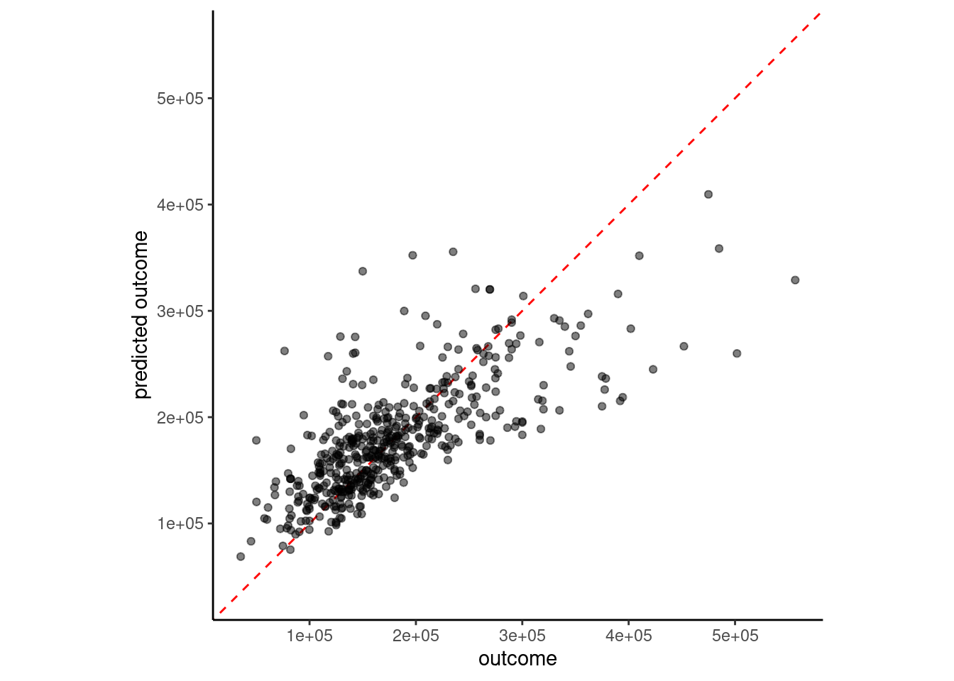

Perfect performance would have all the points right on the dotted line (same value for actual and predicted outcome)

Our model doesn’t do that well yet. Not surprising
Pattern also has some indication of fanning of residuals AND some non-linearity with higher outcome scores that suggests need for a power transformation of outcome (e.g., log)
This is consistent with our earlier modeling EDA
Perhaps not that bad here b/c both sale_price and gr_liv_area were positively skewed
We will need consider this eventually

We can quantify model performance by selecting a performance metric

The yardstick package within the tidymodels framework supports calculation of many performance metrics for regression and classification models
See the list of all currently available metrics

Root mean square error (RMSE) is a common performance metric for regression models

You focused on a related metric, sum of squared error (SSE), in PSY 610/710
RMSE simply divides SSE by N (to get mean squared error; MSE) and then takes the square root to return the metric to the original units for the outcome variable
It is easy to calculate using rmse_vec() from the yardstick package

rmse_vec(truth = feat_val$sale_price, 
         estimate = predict(fit_lm_1, feat_val)$.pred)

[1] 51375.08

Let’s record how well this model performed in validation so we can compare it to subsequent models

error_val <- bind_rows(error_val, 
                       tibble(model = "simple linear model", 
                              rmse_val = rmse_vec(truth = feat_val$sale_price, 
                                                  estimate = predict(fit_lm_1,
                                                                     feat_val)$.pred)))
error_val

# A tibble: 1 × 2
  model               rmse_val
  <chr>                  <dbl>
1 simple linear model   51375.

NOTE: I will continue to bind RMSE to this dataframe for newer models but plan to hide this code chuck to avoid distractions. You can reuse this code repeatedly to track your own models if you like. (Perhaps we should write a function??)

For explanatory purposes, we might want to visualize the relationship between a feature and the outcome (in addition to examining the parameter estimates and the associated statistical tests)

Here is a plot of $\hat{sale\_price}$ by gr_liv_area superimposed over a scatterplot of the raw data from the validation set

feat_val |> 
  ggplot(aes(x = gr_liv_area)) +
    geom_point(aes(y = sale_price), color = "gray") +
    geom_line(aes(y = predict(fit_lm_1, data_val)$.pred), 
              linewidth = 1.25, color = "blue") + 
    ggtitle("Validation Set")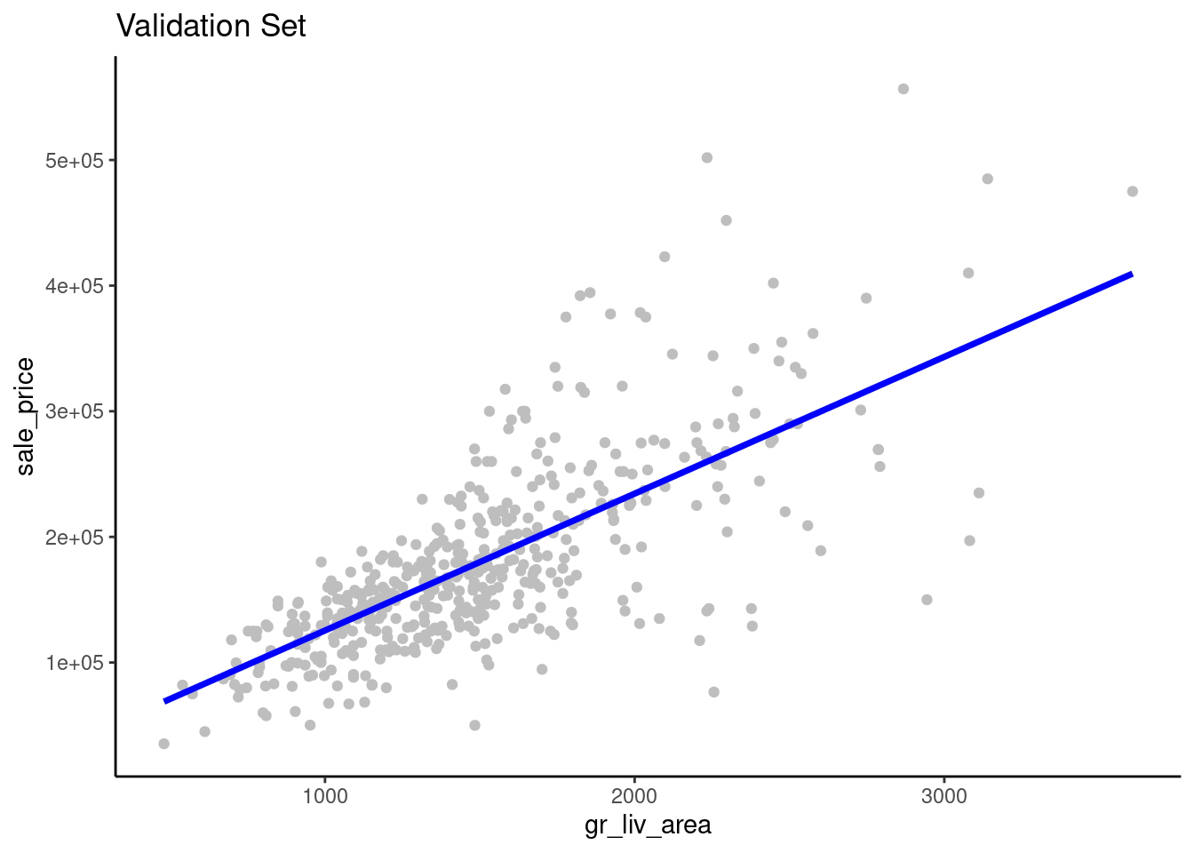

As expected, there is a moderately strong positive relationship between gr_liv_area and sale_price.
We can also again see the heteroscadasticity in the errors that might be corrected by a power transformation of sale_price (or gr_liv_area)

3.3 Extension of LM to Multiple Predictors

We can improve model performance by moving from simple linear model to a linear model with multiple features derived from multiple predictors

We have many other numeric variables available to use, even in this pared down version of the dataset.

data_trn |>  names()

 [1] "sale_price"   "gr_liv_area"  "lot_area"     "year_built"   "overall_qual"
 [6] "garage_cars"  "garage_qual"  "ms_zoning"    "lot_config"   "bldg_type"

Let’s expand our model to also include lot_area, year_built, and garage_cars

Again, we need:

A feature engineering recipe
Training (and eventually validation) feature matrices
An algorithm to fit in training feature matrix

With the addition of new predictors, we now have a feature engineering task

We have missing data on garage_cars in the training set
We need to decide how we will handle it

A simple solution is to do median imputation - substitute the median of the non-missing scores for any missing score.

This is fast and easy to understand
It works OK (but there are certainly better options that we will consider later in the course)
- see other options in Step Functions - Imputation section on tidymodels website
There is only one missing value so it likely doesn’t matter much anyway

Let’s add this to our recipe. All of the defaults are appropriate but you should see ?step_impute_median() to review them

rec <- 
1  recipe(sale_price ~ gr_liv_area + lot_area + year_built + garage_cars,
         data = data_trn) |> 
  step_impute_median(garage_cars)

1: Notice we now list four predictors for our recipe using + between them

Now we need to

First prep recipe

rec_prep <- rec |> 
1  prep(data_trn)

1: I am going to stop using training = at this point. Remember, we prep recipes with training data.

Next, bake the training data with prepped recipe to get training features

feat_trn <- rec_prep |> 
1  bake(data_trn)

1: I am going to stop using new_data = but remember, we use NULL if we want the previously saved training features. If instead, we want features for new data, we provide that dataset.

And take a quick look at the features
- Sample size is correct
- 4 features and the outcome variable
- All features are numeric
- No missing data for garage_qual

feat_trn |> skim_all()

Data summary
Name	feat_trn
Number of rows	1465
Number of columns	5
_______________________
Column type frequency:
numeric	5
________________________
Group variables	None

Variable type: numeric

skim_variable	complete_rate	mean	sd	p0	p25	p50	p75	p100	skew	kurtosis
gr_liv_area	1	1506.84	511.44	438	1128	1450	1759	5642	1.43	5.19
lot_area	1	10144.16	8177.55	1476	7500	9375	11362	164660	11.20	182.91
year_built	1	1971.35	29.65	1880	1953	1972	2000	2010	-0.54	-0.62
garage_cars	1	1.78	0.76	0	1	2	2	4	-0.26	0.10
sale_price	1	180696.15	78836.41	12789	129500	160000	213500	745000	1.64	4.60

And finally, bake the validation data with the same prepped recipe to get validation features

feat_val <- rec_prep |> 
1  bake(data_val)

1: Notice that here we are now baking data_val

And take a quick look
- Correct sample size (N = 490)
- 4 features and outcome
- All numeric
- No missing data

feat_val |> skim_all()

Data summary
Name	feat_val
Number of rows	490
Number of columns	5
_______________________
Column type frequency:
numeric	5
________________________
Group variables	None

Variable type: numeric

skim_variable	complete_rate	mean	sd	p0	p25	p50	p75	p100	skew	kurtosis
gr_liv_area	1	1493.00	483.78	480	1143.5	1436.0	1729.50	3608	0.92	1.16
lot_area	1	10462.08	10422.55	1680	7500.0	9563.5	11780.75	215245	15.64	301.66
year_built	1	1971.08	30.96	1875	1954.0	1975.0	2000.00	2010	-0.66	-0.41
garage_cars	1	1.74	0.76	0	1.0	2.0	2.00	4	-0.24	0.22
sale_price	1	178512.82	75493.59	35311	129125.0	160000.0	213000.00	556581	1.42	2.97

Now let’s combine our algorithm and training features to fit this model configuration with 4 features

fit_lm_4 <- 
  linear_reg() |> 
  set_engine("lm") |> 
1  fit(sale_price ~ ., data = feat_trn)

1: the . is a bit more useful now

This yields these parameter estimates (which as we know from 610/710 were selected to minimize SSE in the training set):

fit_lm_4 |> tidy()

# A tibble: 5 × 5
  term            estimate std.error statistic   p.value
  <chr>              <dbl>     <dbl>     <dbl>     <dbl>
1 (Intercept) -1665041.    89370.       -18.6  1.14e- 69
2 gr_liv_area       76.8       2.62      29.3  3.56e-149
3 lot_area           0.514     0.146      3.51 4.60e-  4
4 year_built       854.       46.2       18.5  7.66e- 69
5 garage_cars    22901.     1964.        11.7  4.09e- 30

Here is our parametric model

$\hat{sale\_price} = -1.6650409\times 10^{6} + 76.8 * gr\_liv\_area + 0.5 * lot\_area + 854.3 * year\_built + 2.29008\times 10^{4} * garage\_cars$

Compared with our previous simple regression model:

$\hat{sale\_price} = 1.6561\times 10^{4} + 108.9 * gr\_liv\_area$

Of course, these four features are correlated both with sale_price but also with each other

Let’s look at correlations in the training set.

feat_trn |> 
  cor() |> 
  corrplot::corrplot.mixed()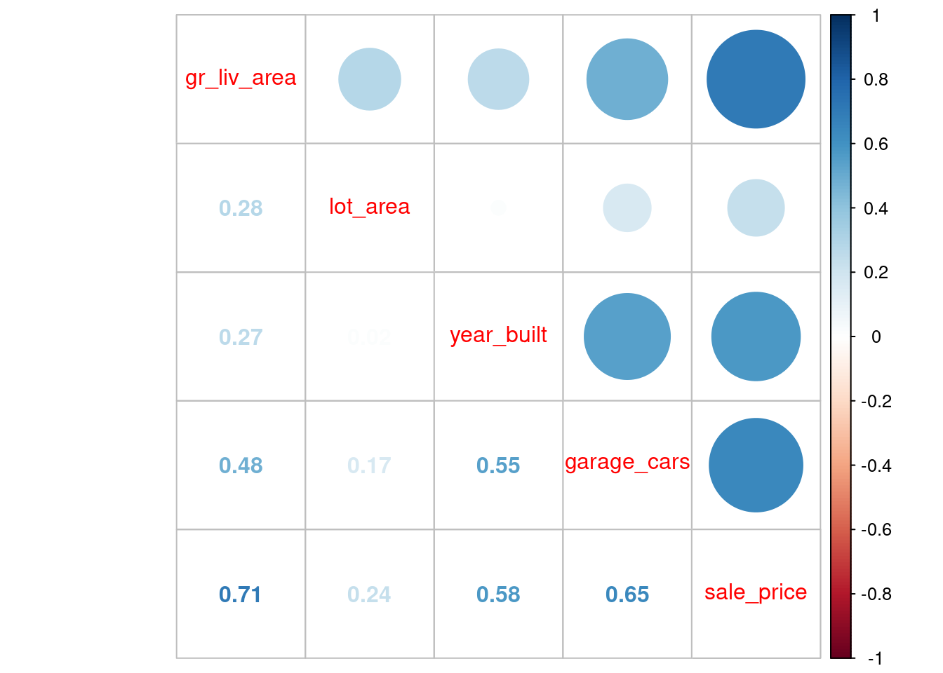

Question: What are the implications of the correlations among many of these predictors?

Show Answer

The multiple regression model coefficients represent unique effects, controlling for 
all other variables in the model.  You can see how the unique effect of `gr_liv_area` 
is smaller than its overall effect from the simple regression.   This also means 
that the overall predictive strength of the model will not be a sum of the effects 
of each predictor considered in isolation - it will likely be less.  Also, if the 
correlations are high, problems with multicollinearity will emerge.  This will yield 
large standard errors which means that the models will start to have more variance when 
fit in different training datasets!  We will soon learn about other regularized 
versions of the GLM that do not have these issues with correlated predictors.

How well does this more complex model perform in validation? Let’s compare the previous and current visualizations of $sale\_price$ vs. $\hat{sale\_price}$

Looks like the errors are smaller (closer to the diagonal line that would represent prefect prediction)
Clear signs of non-linearity are now present as well. Time for more Modeling EDA!!

plot_1 <- plot_truth(truth = feat_val$sale_price, 
                     estimate = predict(fit_lm_1, feat_val)$.pred)

plot_4 <- plot_truth(truth = feat_val$sale_price, 
                     estimate = predict(fit_lm_4, feat_val)$.pred)

cowplot::plot_grid(plot_1, plot_4, 
          labels = list("1 feature", "4 features"), hjust = -1.5)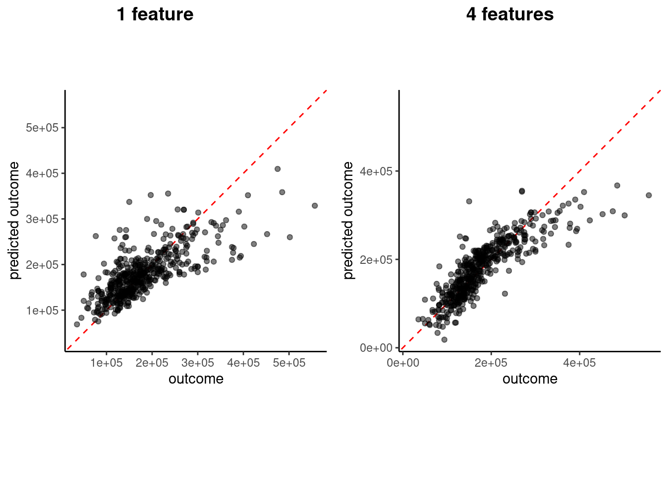

Coding sidebar: Notice the use of plot_grid() from the cowplot package to make side by side plots. This also required returning the individual plots as objects (just assign to a object name, e.g., plot_1)

Let’s compare model performance for the two models using RMSE in the validation set

The one feature simple linear model

rmse_vec(feat_val$sale_price, 
         predict(fit_lm_1, feat_val)$.pred)

[1] 51375.08

The four feature linear model. A clear improvement!

rmse_vec(feat_val$sale_price, 
         predict(fit_lm_4, feat_val)$.pred)

[1] 39903.25

Let’s bind the new performance metric to our results table

# A tibble: 2 × 2
  model                  rmse_val
  <chr>                     <dbl>
1 simple linear model      51375.
2 4 feature linear model   39903.

Given the non-linearity suggested by the truth vs. estimate plots, we might wonder if we could improve the fit if we transformed our features to be closer to normal

There are a number of recipe functions that do transformations (see Step Functions - Individual Transformations)
We will apply step_YeoJohnson(), which is similar to a Box-Cox transformation but can be more broadly applied because the scores don’t need to be strictly positive

Let’s do it all again, now with transformed features!

Define the feature engineering recipe

rec <- 
  recipe(sale_price ~ gr_liv_area + lot_area + year_built + garage_cars, 
         data = data_trn) |> 
  step_impute_median(garage_cars) |> 
  step_YeoJohnson(lot_area, gr_liv_area, year_built, garage_cars)

Prep the recipe with training set

rec_prep <- rec |> 
  prep(data_trn)

Use prepped recipe to bake the training set into features
Notice the features are now less skewed (but sale_price is still skewed)

feat_trn <- rec_prep |> 
  bake(NULL)

feat_trn |> skim_all()

Data summary
Name	feat_trn
Number of rows	1465
Number of columns	5
_______________________
Column type frequency:
numeric	5
________________________
Group variables	None

Variable type: numeric

skim_variable	complete_rate	mean	sd	p0	p25	p50	p75	p100	skew	kurtosis
gr_liv_area	1	5.22	0.16	4.60	5.11	5.23	5.33	5.86	0.00	0.12
lot_area	1	14.10	1.14	10.32	13.69	14.20	14.64	21.65	0.08	5.46
year_built	1	1971.35	29.65	1880.00	1953.00	1972.00	2000.00	2010.00	-0.54	-0.62
garage_cars	1	2.12	0.98	0.00	1.11	2.37	2.37	5.23	-0.03	0.04
sale_price	1	180696.15	78836.41	12789.00	129500.00	160000.00	213500.00	745000.00	1.64	4.60

Use same prepped recipe to bake the validation set into features
Again, features are less skewed

feat_val <- rec_prep |> 
  bake(data_val)

feat_val |> skim_all()

Data summary
Name	feat_val
Number of rows	490
Number of columns	5
_______________________
Column type frequency:
numeric	5
________________________
Group variables	None

Variable type: numeric

skim_variable	complete_rate	mean	sd	p0	p25	p50	p75	p100	skew	kurtosis
gr_liv_area	1	5.22	0.16	4.65	5.11	5.23	5.32	5.66	-0.17	0.19
lot_area	1	14.14	1.17	10.57	13.69	14.24	14.72	22.44	0.11	6.12
year_built	1	1971.08	30.96	1875.00	1954.00	1975.00	2000.00	2010.00	-0.66	-0.41
garage_cars	1	2.06	0.96	0.00	1.11	2.37	2.37	5.23	0.01	0.24
sale_price	1	178512.82	75493.59	35311.00	129125.00	160000.00	213000.00	556581.00	1.42	2.97

Fit model

fit_lm_4yj <- 
  linear_reg() |> 
  set_engine("lm") |> 
  fit(sale_price ~ ., data = feat_trn)

View truth vs. estimate plot

plot_truth(truth = feat_val$sale_price,
           estimate = predict(fit_lm_4yj, feat_val)$.pred)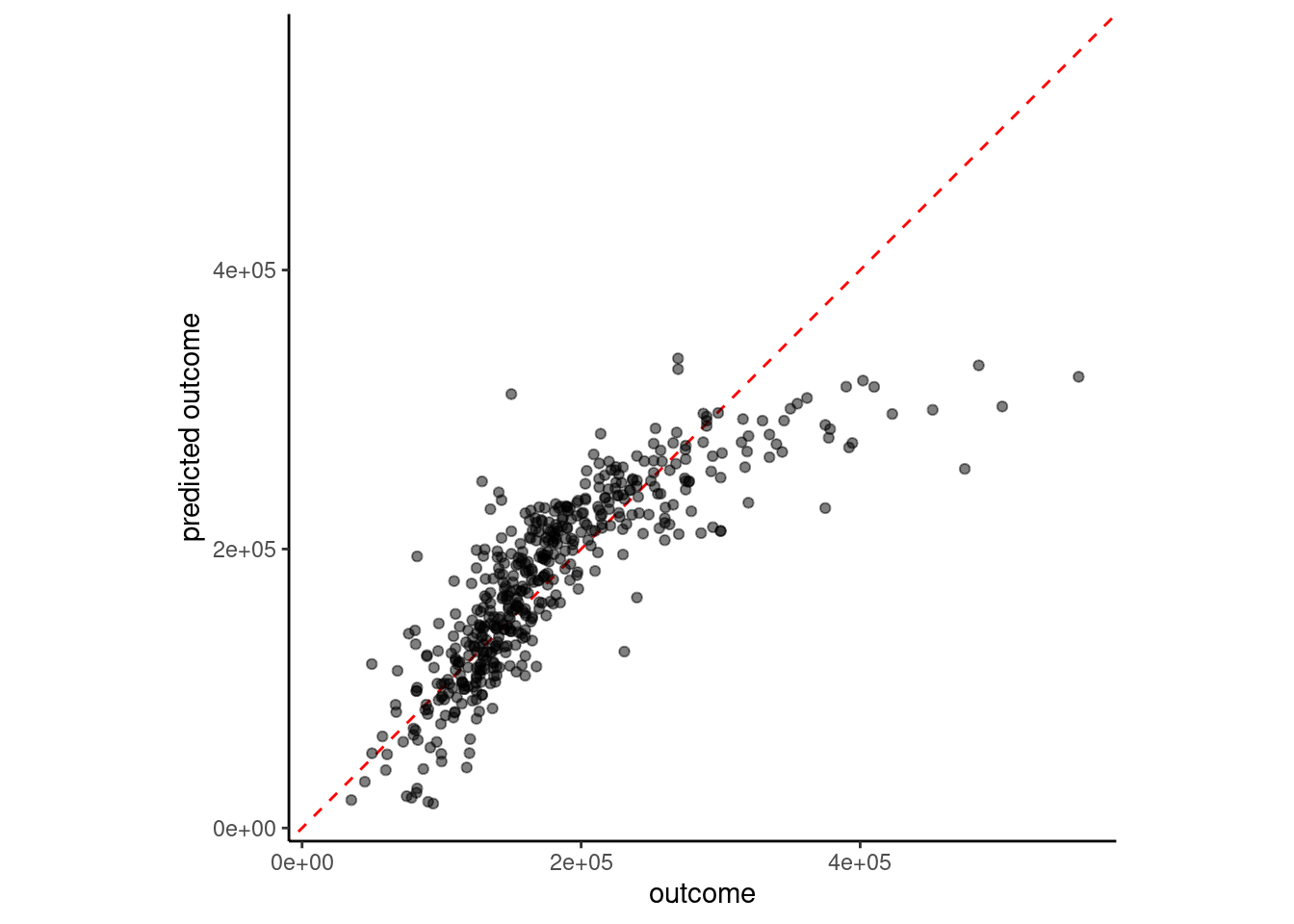

and look at the error

# A tibble: 3 × 2
  model                          rmse_val
  <chr>                             <dbl>
1 simple linear model              51375.
2 4 feature linear model           39903.
3 4 feature linear model with YJ   41660.

That didn’t help at all. Error still high and still non-linearity in plot.

We may need to consider

a transformation of sale_price (We will leave that to you for the application assignment if you are daring!)
or a different algorithm that can handle non-linear relationships better

3.4 Extension to Categorical Predictors

Many important predictors in our models may be categorical (nominal and some ordinal predictors)

Some statistical algorithms (e.g., random forest) can accept even nominal predictors as features without any further feature engineering
But many cannot. Linear models cannot.
The type of feature engineering may differ for nominal vs. ordinal categorical predictors
For nominal categorical predictors:
- We need to learn a common approach to transform them to numeric features - dummy coding. We will learn the concept in general AND how to accomplish within a feature engineering recipe.
For ordinal predictors:
- We can treat them like numeric predictors
- We can treat them like nominal categorical predictors
See article on Categorical Predictors on the tidymodels website for more details

3.4.1 Dummy Coding

For many algorithms, we will need to use feature engineering to convert a categorical predictor to numeric features. One common technique is to use dummy coding. When dummy coding a predictor, we transform the original categorical predictor with m levels into m-1 dummy coded features.

To better understand how and why we do this, lets consider a version of ms_zoning in the Ames dataset.

data_trn |> 
  pull(ms_zoning) |> 
  table()


    agri   commer    float    indus res_high  res_low  res_med 
       2       13       66        1        9     1157      217

We will recode ms_zoning to have only 3 levels to make our example simple (though dummy codes can be used for predictors with any number of levels)

data_dummy <- data_trn |> 
1  select(sale_price, ms_zoning)  |>
2  mutate(ms_zoning3 = fct_collapse(ms_zoning,
                                 "residential" = c("res_high", "res_med",
                                                   "res_low"),
                                 "commercial" = c("agri", "commer", "indus"),
3                                 "floating" = "float")) |>
4  select(-ms_zoning)

1: Make a df (dataframe) with only sale_price and ms_zoning
2: fct_collapse() from the forcats package is our preferred way to collapse levels of a factor. See fct_recode() for more generic recoding of levels.
3: We could have left this line out and float would have stayed as a level named float
4: Remove original ms_zoning predictor

Take a look at the new predictor

data_dummy |> 
  pull(ms_zoning3) |> 
  table()


 commercial    floating residential 
         16          66        1383

Question: Why can’t we simply recode each level with a different consecutive value (e.g., commercial = 1, floating =2 , residential = 3)?

Show Answer

There is no meaningful way to order the numbers that we assign to the levels of 
this unordered categorical predictor.  The shape and strength of the relationship
between it and sale_price will completely change based on arbitrary ordering of 
the levels.

Imagine fitting a straight line to predict sale_price from ms_zoning3 using these three different ways to arbitrarily assign numbers to levels.

data_dummy |> 
  mutate(ms_zoning3 = case_when(ms_zoning3 == "residential" ~ 1,
                                ms_zoning3 == "commercial" ~ 2,
                                ms_zoning3 == "floating" ~ 3)) |> 
  ggplot(aes(x = ms_zoning3, y = sale_price)) +
    geom_bar(stat="summary", fun = "mean")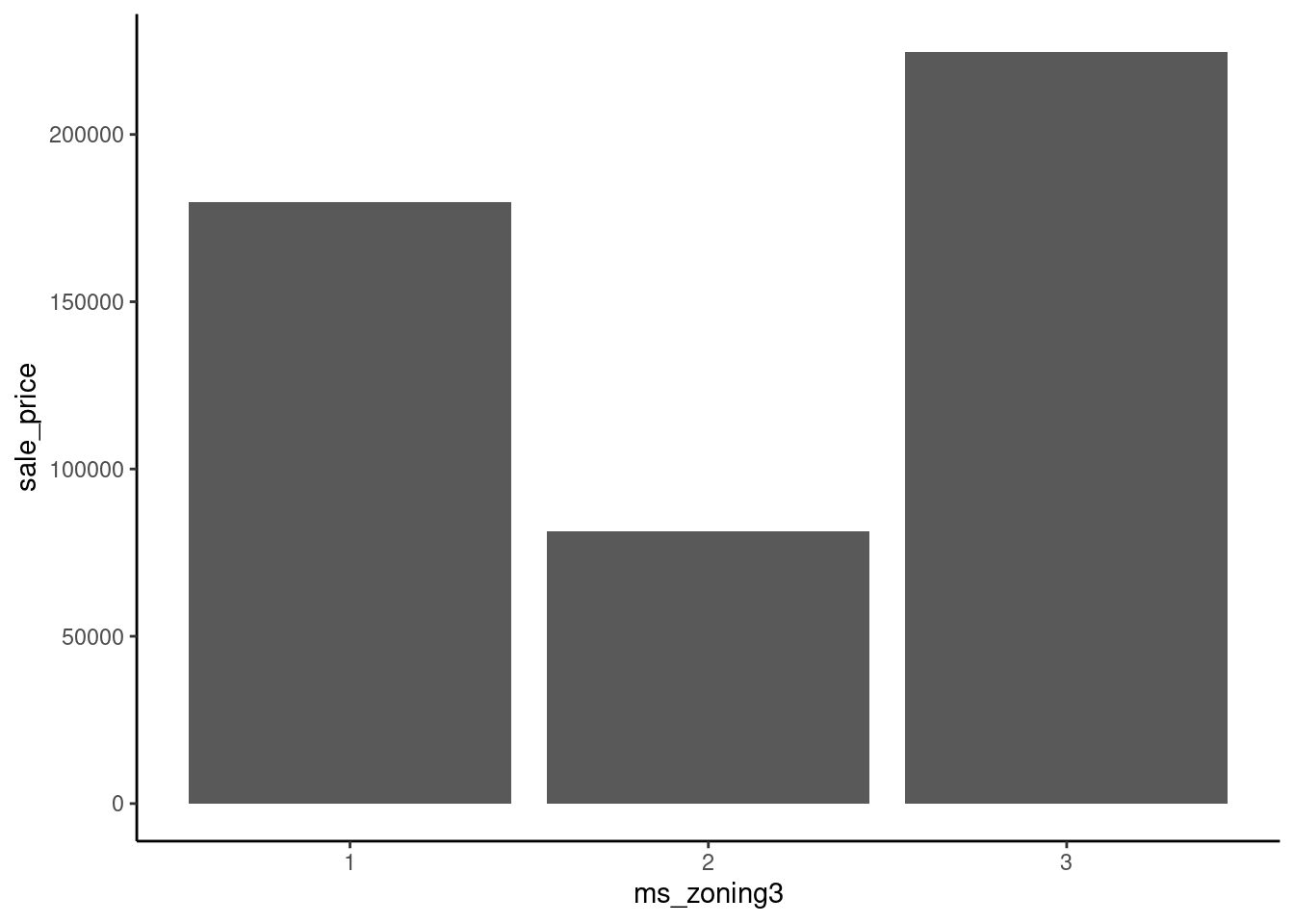

data_dummy |> 
  mutate(ms_zoning3 = case_when(ms_zoning3 == "residential" ~ 2,
                                ms_zoning3 == "commercial" ~ 1,
                                ms_zoning3 == "floating" ~ 3)) |> 
  ggplot(aes(x = ms_zoning3, y = sale_price)) +
    geom_bar(stat="summary", fun = "mean")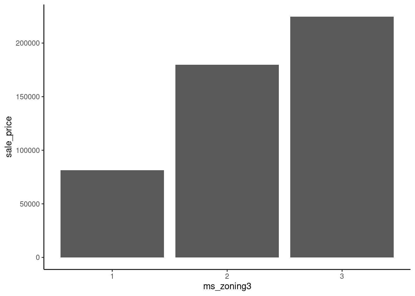

data_dummy |> 
  mutate(ms_zoning3 = case_when(ms_zoning3 == "residential" ~ 3,
                                ms_zoning3 == "commercial" ~ 1,
                                ms_zoning3 == "floating" ~ 2)) |> 
  ggplot(aes(x = ms_zoning3, y = sale_price)) +
    geom_bar(stat="summary", fun = "mean")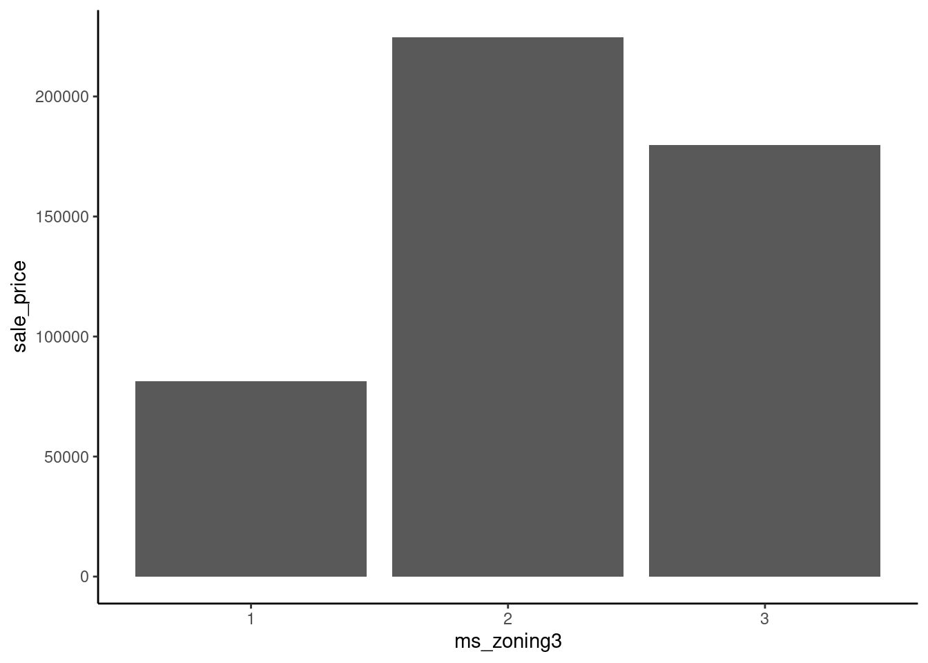

Dummy coding resolves this issue.

When using dummy codes, we transform (i.e., feature engineer) our original m-level categorical predictor to m-1 dummy features.
Each of these m-1 features represents a contrast between a specific level of the categorical variable and a reference level
The full set of m-1 features represents the overall effect of the categorical predictor variable.
We assign values of 0 or 1 to each observation on each feature in a meaningful pattern (see below)

For example, with our three-level predictor: ms_zoning3

We need 2 dummmy features (d1, d2) to represent this 3-level categorical predictor
Dummy feature 1 is coded 1 for residential and 0 for all other levels
Dummy feature 2 is coded 1 for floating and 0 for all other levels

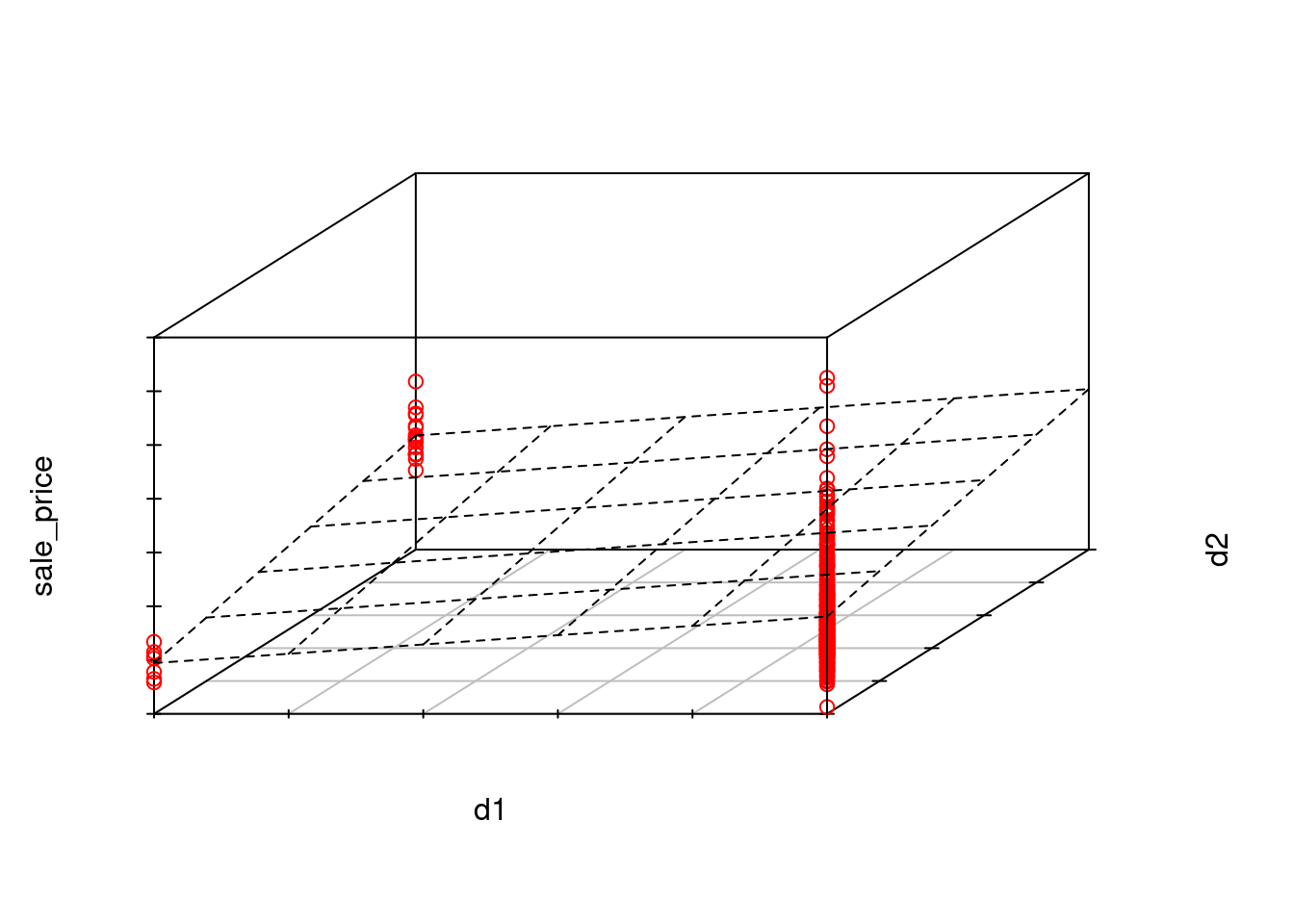
Here is this coding scheme displayed in a table

# A tibble: 3 × 3
  ms_zoning3     d1    d2
  <chr>       <dbl> <dbl>
1 commercial      0     0
2 residential     1     0
3 floating        0     1

With this coding:

Commercial properties are coded 0 for both d1 and d2.
This means that commercial properties will become the reference level against which both residential and floating village are compared.
Because we are focused on prediction, the choice of reference level is mostly arbitrary. For explanatory goals, you might consider which level is best suited to be the reference.
There is much deeper coverage of dummy and other contrast coding in 610/710

We can add these two features manually to the data frame and view a handful of observations to make this coding scheme more concrete

# A tibble: 8 × 4
  sale_price ms_zoning3     d1    d2
       <dbl> <fct>       <dbl> <dbl>
1     105000 residential     1     0
2     126000 residential     1     0
3      13100 commercial      0     0
4     115000 residential     1     0
5     149500 floating        0     1
6      40000 commercial      0     0
7     120000 residential     1     0
8     151000 floating        0     1

If we now fit a model where we predict sale_price from these two dummy coded features, each feature would represent the contrast of the mean sale_price for the level coded 1 vs. the mean sale_price for the level that is coded 0 for all features (i.e., commercial)

d1 is the contrast of mean sale_price for residential vs. commercial
d2 is the contrast of mean sale_price for floating vs. commercial
The combined effect of these two features represents the overall effect of ms_zoning3 on sale_price

Lets do this quickly in base R using lm() as you have done previously in 610.

m <- lm(sale_price ~ d1 + d2, data = data_dummy) 

m |> summary()


Call:
lm(formula = sale_price ~ d1 + d2, data = data_dummy)

Residuals:
    Min      1Q  Median      3Q     Max 
-166952  -50241  -20241   31254  565259 

Coefficients:
            Estimate Std. Error t value Pr(>|t|)    
(Intercept)    81523      19409   4.200 2.83e-05 ***
d1             98219      19521   5.031 5.47e-07 ***
d2            143223      21634   6.620 5.03e-11 ***
---
Signif. codes:  0 '***' 0.001 '**' 0.01 '*' 0.05 '.' 0.1 ' ' 1

Residual standard error: 77640 on 1462 degrees of freedom
Multiple R-squared:  0.03151,   Adjusted R-squared:  0.03018 
F-statistic: 23.78 on 2 and 1462 DF,  p-value: 6.858e-11

The mean sale price of residential properties is 9.8219^{4} dollars higher than commercial properties.
The mean sale price of floating villages is 1.43223^{5} dollars higher than commercial properties.

To understand this conceptually, it is easiest to visualize the linear model that would predict sale_price with these two dichotomous features.

There are only three columns of sale_price because the only possible values for d1 and d2 (which are both dichotomous) are
- 0,0 (commercial)
- 1,0 (residential)
- 0,1 (floating village)
This regression with two features yields a prediction plane (displayed)
The left/right tilt of the plane will be the parameter estimate for d1 and it is the contrast of residential vs. commercial
The front/back tilt of the plane will be the parameter estimate for d2 and it is the contrast of floating village vs. commercial

Statistical sidebar:

Any full rank (# levels - 1) set of features regardless of coding system predicts exactly the same (e.g., dummy, helmert, contrast coding)
Preference among coding systems is simply to get single df contrasts of theoretical importance (i.e., for explanation rather than prediction)
Final (m^th) dummy feature is not included b/c its is completely redundant (perfectly multicollinear) with other dummy features. This would also prevent a linear model from fitting (‘dummy variable trap’).
However, some statistical algorithms do not have problems with perfect multicollinearity (e.g., LASSO, ridge regression).
- For these algorithms, you will sometimes see modified version of dummy coding called one-hot coding.
- This approach uses one additional dummy coded feature for the final category.
- We won’t spend time on this but you should be familiar with the term b/c it is often confused with dummy coding.

Coding Sidebar

When creating dummy coded features from factors that have levels with infrequent observations, you may occasionally end up with novel levels in your validation or test sets that were not present in your training set.

This will cause you issues.
These issues are mostly resolved if you make sure to explicitly list all possible levels for a factor when classing that factor in the training data, even if the level doesn’t exist in the training data.
We provide more detail on this issue in an appendix.

3.4.2 Nominal Predictors

Now that we understand how to use dummy coding to feature engineer nominal predictors, let’s consider some potentially important ones that are available to us.

We can discuss if any look promising.

Lets return first to ms_zoning

data_trn |> 
  plot_categorical("ms_zoning", "sale_price") |> 
  cowplot::plot_grid(plotlist = _, ncol = 2)

Warning: Groups with fewer than two datapoints have been dropped.
ℹ Set `drop = FALSE` to consider such groups for position adjustment purposes.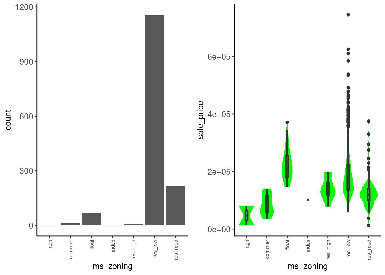

We might:

Represent it with 6 dummy features (because there are 7 raw levels) but many of the categories are very low n - won’t account for much variance?
Combine all the commercial categories (agri, commer, indus), which would take care of most of the low n groups. They also all tend to have the lower prices.
Combine all the residential to get a better feature to variance accounted ratio. They all tend to have similar prices on average and res_high is also pretty low n.

Data dictionary entry: Identifies the general zoning classification of the sale.

agri: Agriculture
commer: Commercial
float: Floating Village Residential
indus: Industrial
res_high: Residential High Density
res_med: Residential Medium Density
res_low: Residential Low Density

lot_config

data_trn |> 
  plot_categorical("lot_config", "sale_price") |> 
  cowplot::plot_grid(plotlist = _, ncol = 2)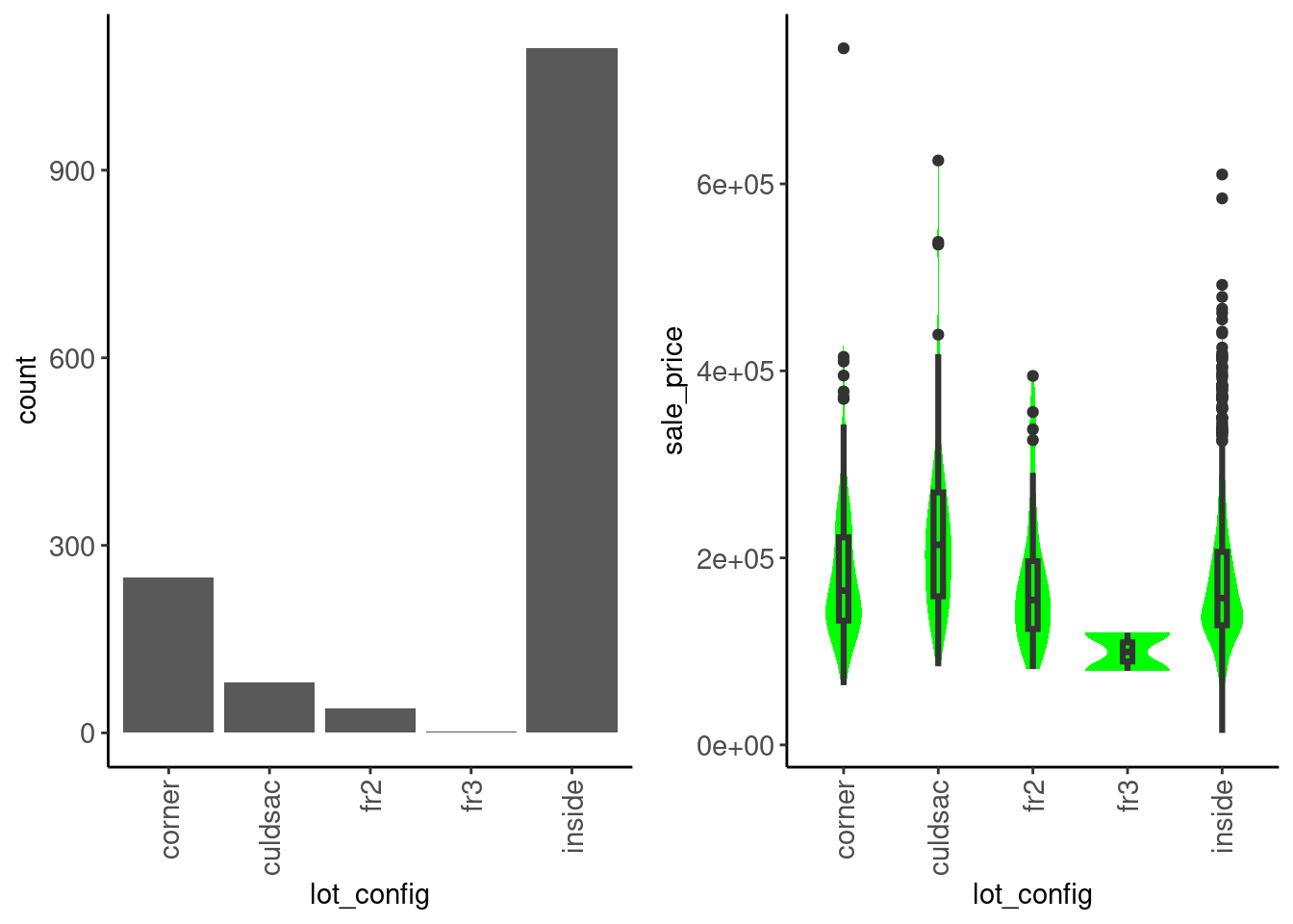

We see that:

Most are inside lots, some of the lot categories are low n
Median sale_price is not very different between configurations
Not very promising but could help some (particularly given the large sample size)

Data dictionary entry: Lot configuration

inside: Inside lot
corner: Corner lot
culdsac: Cul-de-sac
fr2: Frontage on 2 sides of property
fr3: Frontage on 3 sides of property

bldg_type

data_trn |> 
  plot_categorical("bldg_type", "sale_price") |> 
  cowplot::plot_grid(plotlist = _, ncol = 2)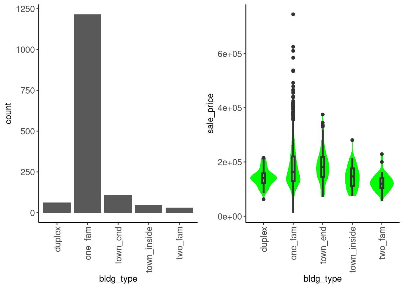

We see that:

Most of the houses are in one category - one_fam
There is not much difference in median sale_price among categories
Not very promising

Data dictionary entry: Type of dwelling

one_fam: Single-family Detached
two_fam: Two-family Conversion; originally built as one-family dwelling
duplex: Duplex
town_end: Townhouse End Unit
town_inside: Townhouse Inside Unit

Let’s do some feature engineering with ms_zoning. We can now do this formally in a recipe so that it can be used in our modeling workflow.

First, if you noticed earlier, there are some levels for ms_zoning that are pretty infrequent. Lets make sure both data_trn and data_val have all levels set for this factor.

data_trn |> pull(ms_zoning) |> levels()

[1] "agri"     "commer"   "float"    "indus"    "res_high" "res_low"  "res_med"

data_val |> pull(ms_zoning) |> levels()

[1] "commer"   "float"    "indus"    "res_high" "res_low"  "res_med"

As expected, we are missing a level (agri) in data_val. Lets fix that here

data_val <- data_val |> 
  mutate(ms_zoning = factor(ms_zoning, 
                            levels = c("agri", "commer", "float", "indus", 
                                       "res_high", "res_low", "res_med")))

[Note: Ideally, you would go back to cleaning EDA and add this level to the full dataset and then re-split into training, validation and test. This is a sloppy shortcut!]

With that fixed, let’s proceed:

We will collapse categories down to three levels (commercial, residential, floating village) as before but now using step_mutate() combined with fct_collapse() to do this inside of our recipe.
We will convert to dummy features using step_dummy(). The first level of the factor will be set to the reference level when we call step_dummy().
step_dummy() is a poor choice for function name. It actually uses whatever contrast coding we have set up in R. However, the default is are dummy coded contrasts (R calls this treatment contrasts). See ?contrasts and options("contrasts") for more info.

rec <- 
  recipe(sale_price ~ gr_liv_area + lot_area + year_built + garage_cars + ms_zoning, 
         data = data_trn) |> 
  step_impute_median(garage_cars) |> 
  step_mutate(ms_zoning = fct_collapse(ms_zoning,
                                 "residential" = c("res_high", "res_med", "res_low"),
                                 "commercial" = c("agri", "commer", "indus"),
                                 "floating" = "float")) |>
  step_dummy(ms_zoning)

Coding Sidebar

You should also read more about some other step_() functions that you might use for categorical predictors: - step_other() to combine all low frequency categories into a single “other” category. - step_unknown() to assign missing values their own category - You can use selector functions. For example, you could make dummy variables out of all of your factors in one step using step_dummy(all_nominal_predictors()).

See the Step Functions - Dummy Variables and Encoding section on the tidymodels website for additional useful functions.

We have also described these in the section on factor steps in Appendix 1

Let’s see if the addition of ms_zoning helped

Notice the addition of the dummy coded features to the feature matrix
Notice the removal of the factor ms_zoning

rec_prep <- rec |> 
  prep(data_trn)

feat_trn <- rec_prep |> 
  bake(NULL)

feat_val <- rec_prep |> 
  bake(data_val)

skim

feat_trn |> skim_all()

Data summary
Name	feat_trn
Number of rows	1465
Number of columns	7
_______________________
Column type frequency:
numeric	7
________________________
Group variables	None

Variable type: numeric

skim_variable	complete_rate	mean	sd	p0	p25	p50	p75	p100	skew	kurtosis
gr_liv_area	1	1506.84	511.44	438	1128	1450	1759	5642	1.43	5.19
lot_area	1	10144.16	8177.55	1476	7500	9375	11362	164660	11.20	182.91
year_built	1	1971.35	29.65	1880	1953	1972	2000	2010	-0.54	-0.62
garage_cars	1	1.78	0.76	0	1	2	2	4	-0.26	0.10
sale_price	1	180696.15	78836.41	12789	129500	160000	213500	745000	1.64	4.60
ms_zoning_floating	1	0.05	0.21	0	0	0	0	1	4.38	17.22
ms_zoning_residential	1	0.94	0.23	0	1	1	1	1	-3.86	12.90

feat_val |> skim_all()

Data summary
Name	feat_val
Number of rows	490
Number of columns	7
_______________________
Column type frequency:
numeric	7
________________________
Group variables	None

Variable type: numeric

skim_variable	complete_rate	mean	sd	p0	p25	p50	p75	p100	skew	kurtosis
gr_liv_area	1	1493.00	483.78	480	1143.5	1436.0	1729.50	3608	0.92	1.16
lot_area	1	10462.08	10422.55	1680	7500.0	9563.5	11780.75	215245	15.64	301.66
year_built	1	1971.08	30.96	1875	1954.0	1975.0	2000.00	2010	-0.66	-0.41
garage_cars	1	1.74	0.76	0	1.0	2.0	2.00	4	-0.24	0.22
sale_price	1	178512.82	75493.59	35311	129125.0	160000.0	213000.00	556581	1.42	2.97
ms_zoning_floating	1	0.05	0.22	0	0.0	0.0	0.00	1	4.07	14.58
ms_zoning_residential	1	0.93	0.25	0	1.0	1.0	1.00	1	-3.51	10.33

Now lets fit a model with these features

fit_lm_6 <- 
  linear_reg() |> 
  set_engine("lm") |> 
  fit(sale_price ~ ., data = feat_trn)

plot it

plot_truth(truth = feat_val$sale_price, 
           estimate = predict(fit_lm_6, feat_val)$.pred)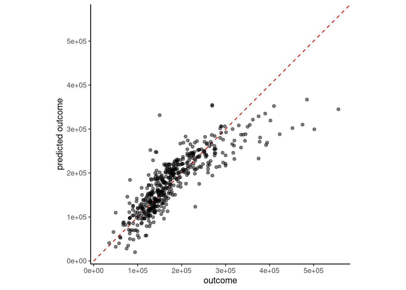

And evaluate it

# A tibble: 4 × 2
  model                              rmse_val
  <chr>                                 <dbl>
1 simple linear model                  51375.
2 4 feature linear model               39903.
3 4 feature linear model with YJ       41660.
4 6 feature linear model w/ms_zoning   39846.

Removing Yeo Johnson transformation but adding dummy coded ms_zoning may have helped a little

Question: Will the addition of new predictors/features to a model always reduce RMSE in train? in validation?

Show Answer

As you know, the estimation procedure in linear models is OLS.  Parameter estimates
are derived to minimize the SSE in the data set in which they are derived.  For this
reason, adding a predictor will never increase RMSE in the training set and it will
usually lower it even when it is not part of the DGP.   However, this is not true in
validation.  A predictor will only meaningfully lower RMSE in validation if it is
part of the DGP.  Also, a bad predictor could even increase RMSE in validation due to
overfitting.

3.4.3 Ordinal Predictors

We have two paths to pursue for ordinal predictors

We can treat them like nominal predictors (e.g., dummy code)
We can treat them like numeric predictors (either raw or with an added transformation if needed)

Let’s consider overall_qual

data_trn |> 
  plot_categorical("overall_qual", "sale_price") |> 
  cowplot::plot_grid(plotlist = _, ncol = 2)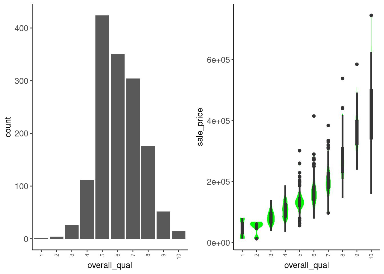

Observations:

Low frequency for low and to some degree high quality response options. If dummy coding, may want to collapse some (1-2)
There is a monotonic relationship (mostly linear) with sale_price. Treat as numeric?
Not skewed so doesn’t likely need to be transformed if treated as numeric
Numeric will take one feature vs. many (9?) features for dummy codes.
Dummy codes are more flexible but we may not need this flexibility (and unnecessary flexibility increases overfitting)

Let’s add overall_qual to our model as numeric

Remember that this predictor was ordinal so we paid special attention to the order of the levels when we classed this factor. Lets confirm they are in order

data_trn |> pull(overall_qual) |> levels()

 [1] "1"  "2"  "3"  "4"  "5"  "6"  "7"  "8"  "9"  "10"

To convert overall_qual to numeric (with levels in the specified order), we can use another simple mutate inside our recipe.

rec <- 
  recipe(sale_price ~  ~ gr_liv_area + lot_area + year_built + garage_cars + 
           ms_zoning + overall_qual, data = data_trn) |> 
  step_impute_median(garage_cars) |> 
  step_mutate(ms_zoning = fct_collapse(ms_zoning,
                                 "residential" = c("res_high", "res_med", "res_low"),
                                 "commercial" = c("agri", "commer", "indus"),
                                 "floating" = "float"),
              overall_qual = as.numeric(overall_qual)) |>
  step_dummy(ms_zoning)

Coding Sidebar

There is a step function called step_ordinalscore() but it requires that the factor is classed as an ordered factor. It is also more complicated than needed in our opinion. Just use as.numeric()

Let’s evaluate this model

Making features
Skipping the skim to save space (we promised we checked it previously!)

rec_prep <- rec |> 
  prep(data_trn)

feat_trn <- rec_prep |> 
  bake(NULL)

feat_val <- rec_prep |> 
  bake(data_val)

Fitting model

fit_lm_7 <- 
  linear_reg() |> 
  set_engine("lm") |> 
  fit(sale_price ~ ., data = feat_trn)

Plotting results

plot_truth(truth = feat_val$sale_price, 
                                 estimate = predict(fit_lm_7, feat_val)$.pred)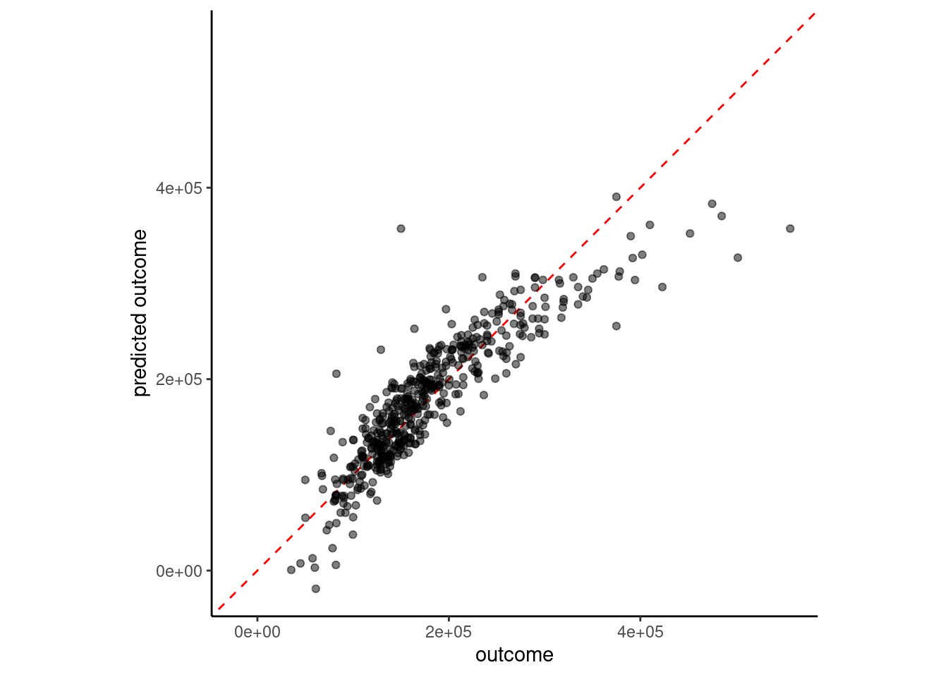

Quantifying held out error

# A tibble: 5 × 2
  model                              rmse_val
  <chr>                                 <dbl>
1 simple linear model                  51375.
2 4 feature linear model               39903.
3 4 feature linear model with YJ       41660.
4 6 feature linear model w/ms_zoning   39846.
5 7 feature linear model               34080.

That helped!

3.5 Extensions to Interactive Models and Non-linear Models

3.5.1 Interactions

There may be interactive effects among our predictors

Some statistical algorithms (e.g., KNN) can naturally accommodate interactive effects without any feature engineering
Linear models cannot
Nothing to fear, tidymodels makes it easy to feature engineer interactions
[BUT - as we will learn, we generally think that if you expect lots of interactions, the linear model may not be the best model to use]

For example, it may be that the relationship between year_built and sale_price depends on overall_qual.

Old houses are expensive if they are in good condition
but old houses are very cheap if they are in poor condition

In the tidymodels framework

Coding interactions is done by feature engineering, not by formula (Note that formula does not change below in recipe)
This seems appropriate to us as we are making new features to represent interactions
We still use an R formula like interface to specify the interaction term features that will be created
see more details on the tidymodels website

rec <- 
  recipe(sale_price ~  ~ gr_liv_area + lot_area + year_built + garage_cars + 
           ms_zoning + overall_qual, data = data_trn) |> 
  step_impute_median(garage_cars) |> 
  step_mutate(ms_zoning = fct_collapse(ms_zoning,
                                 "residential" = c("res_high", "res_med", "res_low"),
                                 "commercial" = c("agri", "commer", "indus"),
                                 "floating" = "float"),
              overall_qual = as.numeric(overall_qual)) |>
  step_dummy(ms_zoning) |> 
  step_interact(~ overall_qual:year_built)

Let’s prep, bake, fit, and evaluate!

rec_prep <- rec |> 
  prep(data_trn)

feat_trn <- rec_prep |> 
  bake(NULL)

feat_val <- rec_prep |> 
  bake(data_val)

Note the new interaction term (we just skim feat_trn here)
Named using “x” to specify the interaction

feat_trn |> skim_all()

Data summary
Name	feat_trn
Number of rows	1465
Number of columns	9
_______________________
Column type frequency:
numeric	9
________________________
Group variables	None

Variable type: numeric

skim_variable	complete_rate	mean	sd	p0	p25	p50	p75	p100	skew	kurtosis
gr_liv_area	1	1506.84	511.44	438	1128	1450	1759	5642	1.43	5.19
lot_area	1	10144.16	8177.55	1476	7500	9375	11362	164660	11.20	182.91
year_built	1	1971.35	29.65	1880	1953	1972	2000	2010	-0.54	-0.62
garage_cars	1	1.78	0.76	0	1	2	2	4	-0.26	0.10
overall_qual	1	6.08	1.41	1	5	6	7	10	0.20	-0.03
sale_price	1	180696.15	78836.41	12789	129500	160000	213500	745000	1.64	4.60
ms_zoning_floating	1	0.05	0.21	0	0	0	0	1	4.38	17.22
ms_zoning_residential	1	0.94	0.23	0	1	1	1	1	-3.86	12.90
overall_qual_x_year_built	1	12015.69	2907.93	1951	9800	11808	14021	20090	0.24	-0.11

fit model

fit_lm_8 <- 
  linear_reg() |> 
  set_engine("lm") |> 
  fit(sale_price ~., 
      data = feat_trn)

plot

plot_truth(truth = feat_val$sale_price, 
           estimate = predict(fit_lm_8, feat_val)$.pred)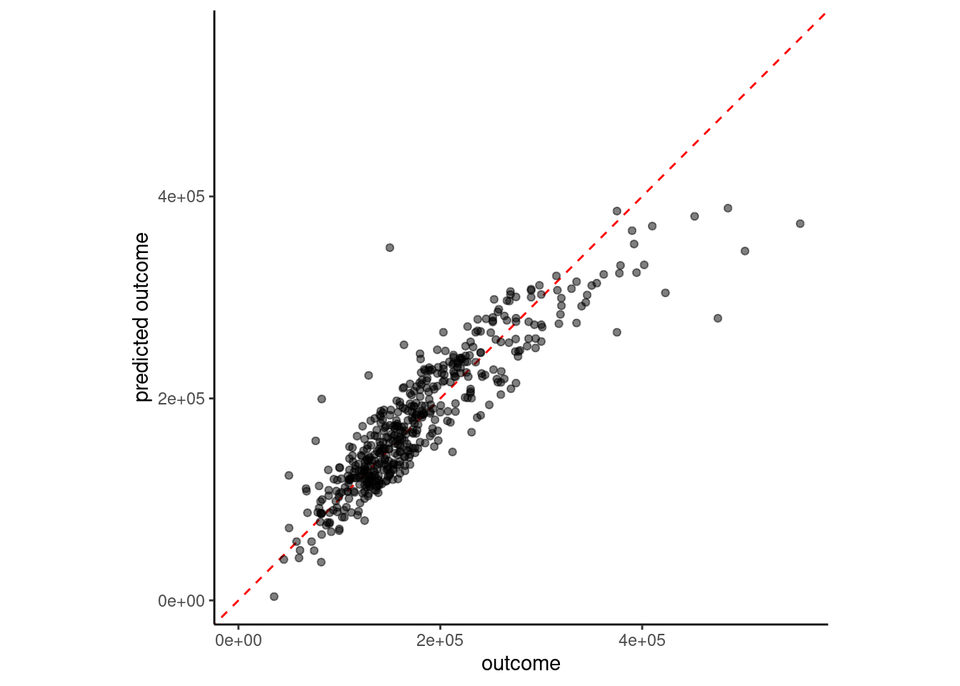

calculate held out error

# A tibble: 6 × 2
  model                                rmse_val
  <chr>                                   <dbl>
1 simple linear model                    51375.
2 4 feature linear model                 39903.
3 4 feature linear model with YJ         41660.
4 6 feature linear model w/ms_zoning     39846.
5 7 feature linear model                 34080.
6 8 feature linear model w/interaction   32720.

That helped!

You can also feature engineer interactions with nominal (and ordinal predictors treated as nominal) predictors

The nominal predictors should first be converted to dummy code features
You will indicate the interactions using the variable names that will be assigned to these dummy code features
Use starts_with() or matches() to make it easy if there are many features associated with a categorical predictor
Can use “~ .^2” to include all two way interactions (be careful if you have dummy coded features!)

Let’s code an interaction between ms_zoning & year_built.

Old homes are cool
Old commercial spaces are never cool
Maybe this is why the main effect of ms_zoning wasn’t useful

rec <- 
  recipe(sale_price ~  ~ gr_liv_area + lot_area + year_built + garage_cars + 
           ms_zoning + overall_qual, data = data_trn) |> 
  step_impute_median(garage_cars) |> 
  step_mutate(ms_zoning = fct_collapse(ms_zoning,
                                 "residential" = c("res_high", "res_med", "res_low"),
                                 "commercial" = c("agri", "commer", "indus"),
                                 "floating" = "float"),
              overall_qual = as.numeric(overall_qual)) |>
  step_dummy(ms_zoning) |> 
  step_interact(~ overall_qual:year_built) |> 
  step_interact(~ starts_with("ms_zoning_"):year_built)

prep, bake

rec_prep <- rec |> 
  prep(data_trn)

feat_trn <- rec_prep |> 
  bake(NULL)

feat_val <- rec_prep |> 
  bake(data_val)

Yup, we have two new interaction features as expected

feat_trn |> skim_all()

Data summary
Name	feat_trn
Number of rows	1465
Number of columns	11
_______________________
Column type frequency:
numeric	11
________________________
Group variables	None

Variable type: numeric

skim_variable	complete_rate	mean	sd	p0	p25	p50	p75	p100	skew	kurtosis
gr_liv_area	1	1506.84	511.44	438	1128	1450	1759	5642	1.43	5.19
lot_area	1	10144.16	8177.55	1476	7500	9375	11362	164660	11.20	182.91
year_built	1	1971.35	29.65	1880	1953	1972	2000	2010	-0.54	-0.62
garage_cars	1	1.78	0.76	0	1	2	2	4	-0.26	0.10
overall_qual	1	6.08	1.41	1	5	6	7	10	0.20	-0.03
sale_price	1	180696.15	78836.41	12789	129500	160000	213500	745000	1.64	4.60
ms_zoning_floating	1	0.05	0.21	0	0	0	0	1	4.38	17.22
ms_zoning_residential	1	0.94	0.23	0	1	1	1	1	-3.86	12.90
overall_qual_x_year_built	1	12015.69	2907.93	1951	9800	11808	14021	20090	0.24	-0.11
ms_zoning_floating_x_year_built	1	90.29	415.84	0	0	0	0	2009	4.38	17.22
ms_zoning_residential_x_year_built	1	1860.03	453.95	0	1948	1968	1997	2010	-3.83	12.78

Fit model

fit_lm_10 <- 
  linear_reg() |> 
  set_engine("lm") |> 
  fit(sale_price ~ ., data = feat_trn)

Plot

plot_truth(truth = feat_val$sale_price, 
           estimate = predict(fit_lm_10, feat_val)$.pred)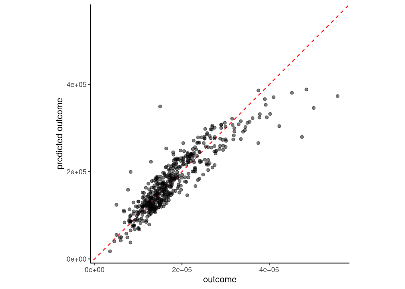

Quantify held out error

error_val <- error_val |> 
  bind_rows(tibble(model = "10 feature linear model w/interactions", 
                   rmse_val = rmse_vec(feat_val$sale_price,
                                       predict(fit_lm_10,
                                               feat_val)$.pred)))

error_val

# A tibble: 7 × 2
  model                                  rmse_val
  <chr>                                     <dbl>
1 simple linear model                      51375.
2 4 feature linear model                   39903.
3 4 feature linear model with YJ           41660.
4 6 feature linear model w/ms_zoning       39846.
5 7 feature linear model                   34080.
6 8 feature linear model w/interaction     32720.
7 10 feature linear model w/interactions   32708.

Not really any better
Shouldn’t just include all interactions without reason
- Either you have done EDA to support them or
- You have substantive interest in them (explanatory question)
- If you want all interactions, use a statistical algorithm that supports those relationships without feature engineering (e.g., KNN, random forest and other decision trees)

3.5.2 Non-linear Models

We may also want to model non-linear effects of our predictors

Some non-parametric models can accommodate non-linear effects without feature engineering (e.g., KNN, Random Forest).
Non-linear effects can be accommodated in a linear model with feature engineering
- Transformations of Y or X. See Step Functions - Individual Transformations on tidymodels website
- Ordinal predictors can be coded with dummy variables
- Numeric predictors can be split at threshold
- Polynomial contrasts for numeric or ordinal predictors (see step_poly())
We will continue to explore these options throughout the course

3.6 KNN Regression

K Nearest Neighbor

Is a non-parametric regression and classification statistical algorithm
- It does not yield specific parameter estimates for features/predictors (or statistical tests for those parameter estimates)
- There are still ways to use it to address explanatory questions (visualizations, model comparisons, feature importance)
Very simple but also powerful (listed commonly among top 10 algorithms)
- By powerful, it is quite flexible and can accommodate many varied DGPs without the need for much feature engineering with its predictors
- May not need most transformations of X or Y
- May not need to model interactions
- Still need to handle missing data, outliers, and categorical predictors

K Nearest Neighbor

Algorithm “memorizes” the training set (lazy learning)
- Lazy learning is most useful for large, continuously changing datasets with few attributes (features) that are commonly queried (e.g., online recommendation systems)
Prediction for any new observation is based on $k$ most similar observations from the dataset
- $k$ provides direct control over the bias-variance trade-off for this algorithm

To better understand KNN let’s simulate training data for three different DGPs (linear - y, polynomial - y2, and step - y3)

Let’s start with a simple example where the DGP for Y is linear on one predictor (X)

DGP: $y = rnorm(150, x, 10)$

This figure displays:

DGP
Prediction line from a simple linear model
Red lines to represent three new observations (X = 10, 50, 90) we want to make predictions for via a standard KNN

Question: What would 5-NN predictions look like for each of these three new values of X in the figure above?

Show Answer

For x = 10, find the five observations that have X values closest to 10.  Average the 
Y values for those 5 observations and that is your predicted Y associated with 
that new value of X.  Repeat to make predictions for Y for any other value of X,
e.g., 50, 90, or any other value

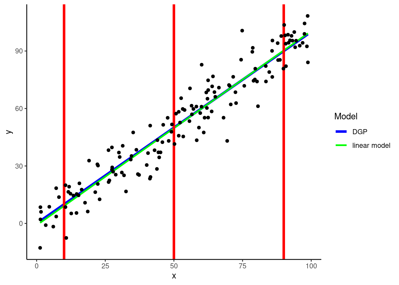
KNN can easily accommodate non-linear relationships between numeric predictors and outcomes without any feature engineering for predictors

In fact, it can flexibly handle any shape of relationship

DGP: $y2 = rnorm(150, x^4 / 800000, 8)$

Warning: Using `size` aesthetic for lines was deprecated in ggplot2 3.4.0.
ℹ Please use `linewidth` instead.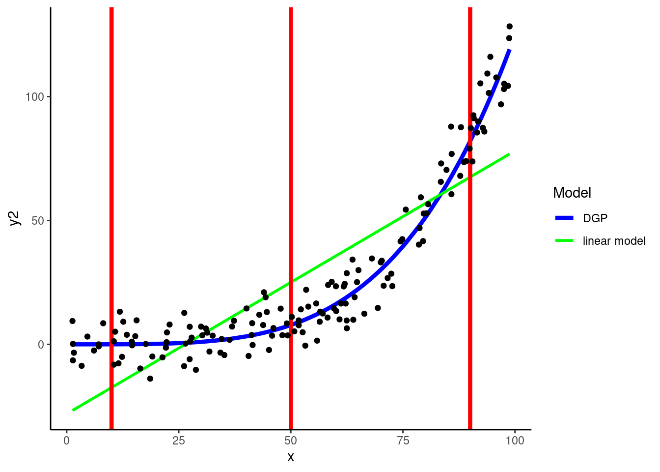

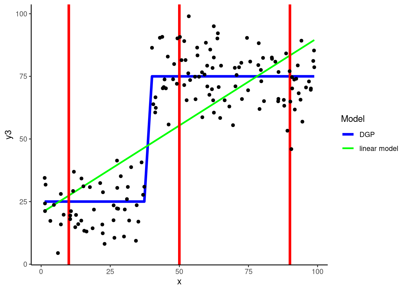
DGP: $y3 = if\_else(x < 40, rnorm(150, 25, 10), rnorm(150, 75, 10))$

3.7 The Hyperparameter k in KNN

KNN is our first example of a statistical algorithm that includes a hyperparameter, in this case $k$

Algorithm hyperparameters differ from parameters in that they cannot be estimated while fitting the algorithm to the training set
They must be set in advance
k = 5 is the default for kknn(), the engine from the kknn package that we will use to fit a KNN within tidymodels.
- $kknn()$ weights observations (neighbors) based on distance.
- An option exists for unweighted as well but not likely used much (default is optimal weighting, use it!).

Using the polynomial DGP above, let’s look at a 5-NN yields

Note the new category of algorithm, new engine, and the need to set a mode (because KNN can be used for regression and classification)
We can look in the package documentation to better understand what is being done (?kknn::train.kknn).

nearest_neighbor() |>   
  set_engine("kknn") |>   
  set_mode("regression") |> 
  translate()

K-Nearest Neighbor Model Specification (regression)

Computational engine: kknn 

Model fit template:
kknn::train.kknn(formula = missing_arg(), data = missing_arg(), 
    ks = min_rows(5, data, 5))

Set up simple feature engineering recipe and get training features (nothing happening but let’s follow normal routine anyway)

rec <- 
  recipe(y2 ~ x, data = data_trn_demo)

rec_prep <- rec |> 
  prep(data_trn_demo)

feat_trn_demo <- rec_prep |> 
  bake(NULL)

Fit 5NN

fit_5nn_demo <- 
  nearest_neighbor() |>   
  set_engine("kknn") |>   
  set_mode("regression") |> 
  fit(y2 ~ ., data = feat_trn_demo)

Get features for a validation set (a new sample using same polynomial DGP)

feat_val_demo <- rec_prep |> 
  bake(data_val_demo)

Display 5NN predictions in validation
- KNN (with k = 5) does a pretty good job of representing the shape of the DGP (low bias)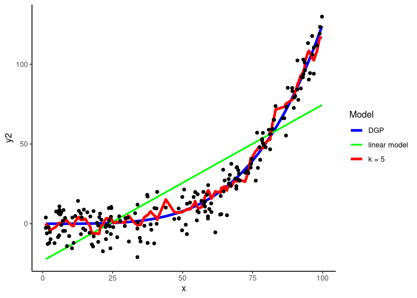
- KNN displays some (but minimal) evidence of overfitting
- Simple linear model does not perform well (clear/high bias)

Let’s pause and consider our conceptual understanding of the impact of $k$ on the bias-variance trade-off

Question: How will the size of k influence model performance (e.g., bias, overfitting/variance)?

Show Answer

Smaller values of k will tend to increase overfitting (and therefore variance 
across training samples) but decrease bias.  Larger values of k will tend to decrease
overfitting but increase bias.  We need to find the Goldilocks "sweet spot"

Question: How will k = 1 perform in training and validation sets?

Show Answer

k = 1 will perfectly fit the training set.  Therefore it is very dependent on the training 
set (high variance).  It will fit both the DGP and the noise in the training set.  
Clearly it will likely not do as well in validation (it will be overfit to training).  
k needs to be larger if there is more noise (to average over more cases).  k needs 
to be smaller if the relationships are complex. (More on choosing k by resampling in 
unit 5.

k = 1

Fit new model
Recipe and features have not changed

fit_1nn_demo <- 
1  nearest_neighbor(neighbors = 1) |>
  set_engine("kknn") |>   
  set_mode("regression") |> 
  fit(y2 ~ ., data = feat_trn_demo)

1: Set k with neighbors =

Visualize prediction models in Train and Validation

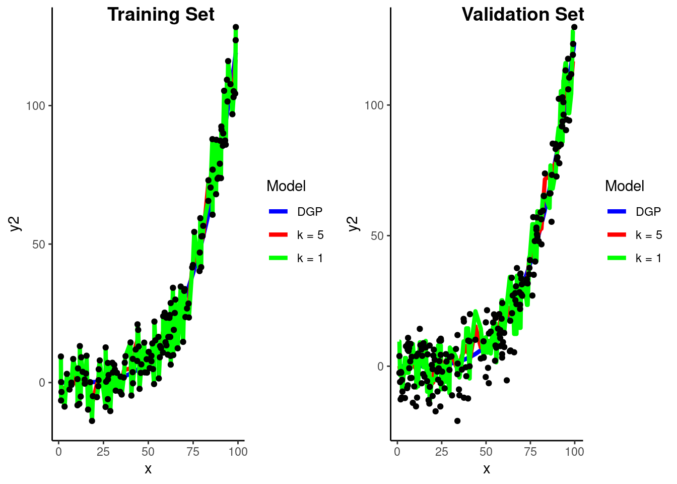
Calculate RMSE in validation for two KNN models

k = 1

rmse_vec(feat_val_demo$y2, 
         predict(fit_1nn_demo, feat_val_demo)$.pred)

[1] 10.91586

k = 5

rmse_vec(feat_val_demo$y2, 
         predict(fit_5nn_demo, feat_val_demo)$.pred)

[1] 8.387035

What if we go the other way and increase $k$ to 75

fit_75nn_demo <- 
  nearest_neighbor(neighbors = 75) |>   
  set_engine("kknn") |>   
  set_mode("regression") |> 
  fit(y2 ~ ., data = feat_trn_demo)

Visualize prediction models in Train and Validation

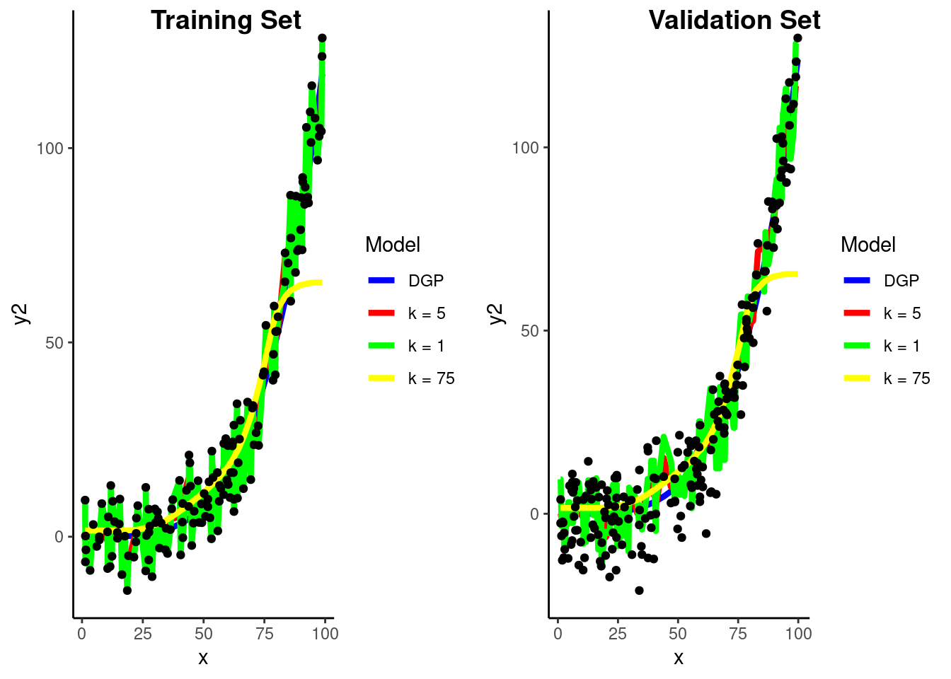
Calculate RMSE in validation for three KNN models

This is the bias-variance trade-off in action

k = 1 - high variance

rmse_vec(feat_val_demo$y2, 
         predict(fit_1nn_demo, feat_val_demo)$.pred)

[1] 10.91586

k = 5 - just right (well better at least)

rmse_vec(feat_val_demo$y2, 
         predict(fit_5nn_demo, feat_val_demo)$.pred)

[1] 8.387035

k = 75 - high bias

rmse_vec(feat_val_demo$y2, 
         predict(fit_75nn_demo, feat_val_demo)$.pred)

[1] 15.34998

3.8 Distance and Scaling in KNN

3.8.1 Defining “Nearest”

To make a prediction for some new observation, we need to identify the observations from the training set that are nearest to it

Need a distance measure to define “nearest”
IMPORTANT: We care only about:
- Distance between a validation observation and all the training observations
- Need to find the $k$ observations in training that are nearest to the validation observation (i.e., its neighbors)
- Distance is defined based on these observations’ features, not their outcomes
There are a number of different distance measures available (e.g., Euclidean, Manhattan, Chebyshev, Cosine, Minkowski)
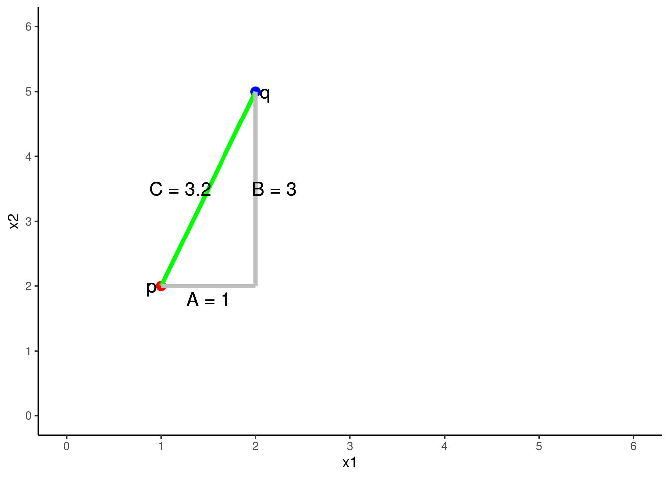
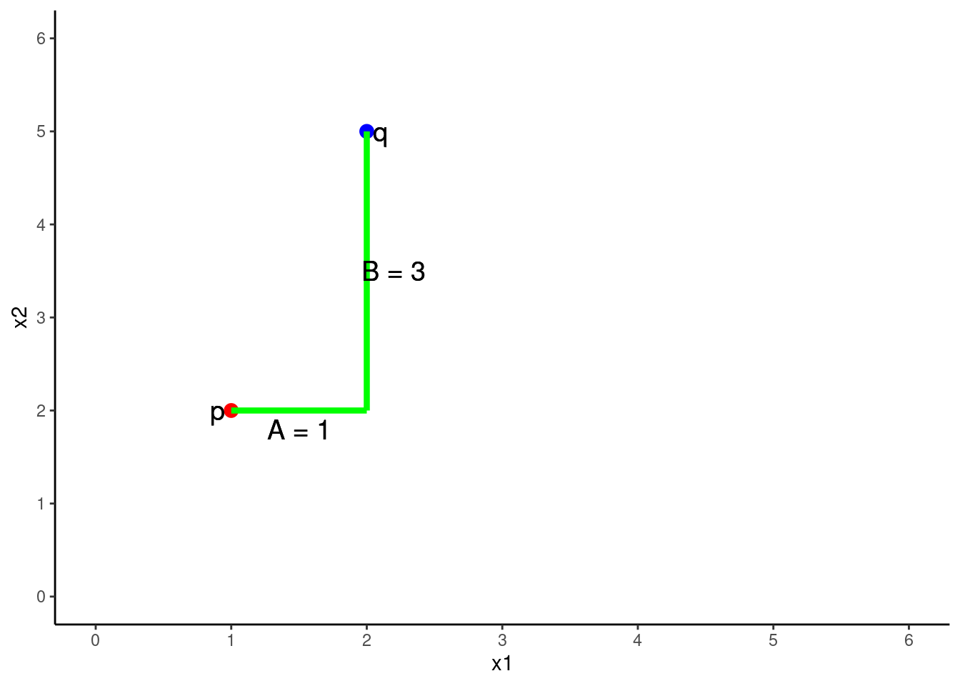
- Euclidean is most commonly used in KNN

Euclidean distance between any two points is an n-dimensional extension of the Pythagorean formula (which applies explicitly with 2 features/2 dimensional space).

$C^2 = A^2 + B^2$

$C = \sqrt{A^2 + B^2}$

…where C is the distance between two points

The Euclidean distance between 2 points (p and q) in two dimensions (2 predictors, x1 = A, x2 = B)

$Distance = \sqrt{A^2 + B^2}$

$Distance = \sqrt{(q1 - p1)^2 + (q2 - p2)^2}$

$Distance = \sqrt{(2 - 1)^2 + (5 - 2)^2}$

$Distance = 3.2$

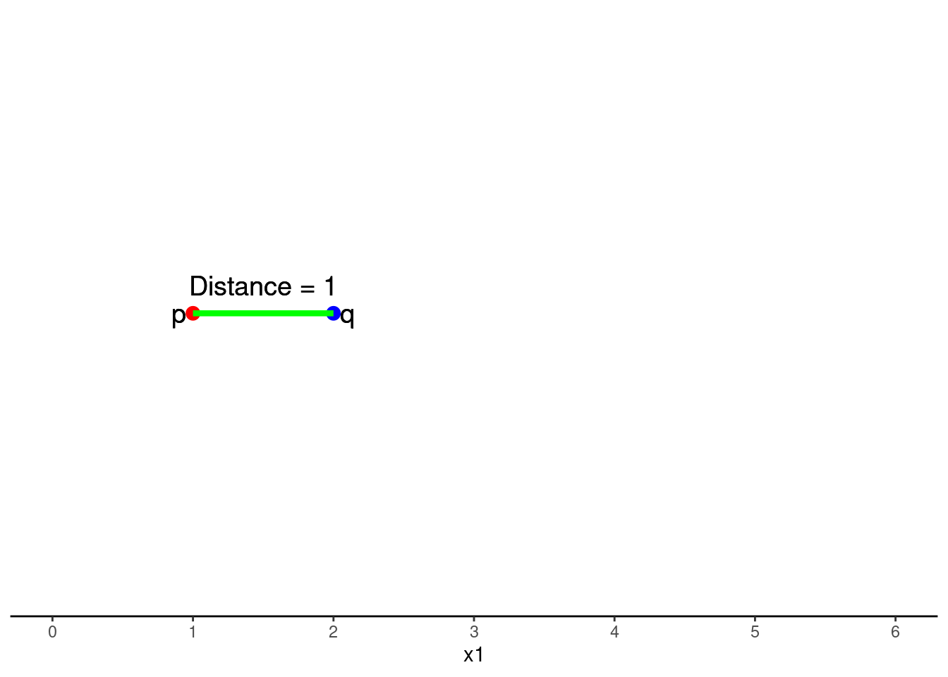
One dimensional (one feature) is simply the subtraction of scores on that feature (x1) between p and q

$Distance = \sqrt{(q1 - p1)^2}$

$Distance = \sqrt{(2 - 1)^2}$

$Distance = 1$

N-dimensional generalization for n features:

$Distance = \sqrt{(q1 - p1)^2 + (q2 - p2)^2 + ... + (qn - pn)^2}$

Manhattan distance is also referred to as city block distance

Travel down the “A” street for 1 unit
Travel down the “B” street for 3 units
Total distance = 4 units

For two features/dimensions

$Distance = |A + B|$

kknn() uses Minkowski distance (see Wikipedia or less mathematical description)

It is a more complex parameterized distance formula
- This parameter is called p, referred to as distance in kknn()
Euclidean and Manhattan distances are special cases where p = 2 and 1, respectively
The default p in kknn() = 2 (Euclidean distance)
This default (like all defaults) can be changed when you define the algorithm using nearest_neighbor()

3.8.2 Scaling X

Distance is dependent on scales of all the features. We need to put all features on the same scale

Scale all features to SD = 1 (using step_scale(all_numeric_predictors()))
Range correct [0, 1] all features (using step_range(all_numeric_predictors()))

3.8.3 Categorical Predictors

KNN requires numeric features (for distance calculation).

For categorical predictors, you will need to use dummy coding or other feature engineering that results in numeric features.
e.g., step_dummy(all_nominal_predictors())

3.9 KNN with Ames Housing Prices

Let’s use KNN with Ames

Train a model using only numeric predictors and overall_qual as numeric
Use the default k = 5 algorithm
Set SD = 1 for all features

rec <- 
  recipe(sale_price ~ gr_liv_area + lot_area + year_built + garage_cars + overall_qual, 
         data = data_trn) |> 
  step_impute_median(garage_cars) |> 
  step_mutate(overall_qual = as.numeric(overall_qual)) |> 
1  step_scale(all_numeric_predictors())

1: Remember to take advantage of these selectors for easier code! See ?has_role for more details

prep, bake

rec_prep <- rec |> 
  prep(data_trn)

feat_trn <- rec_prep |>
  bake(NULL)

feat_val <- rec_prep |> 
  bake(data_val)

Skim training features. Note all SD = 1

feat_trn |> skim_all()

Data summary
Name	feat_trn
Number of rows	1465
Number of columns	6
_______________________
Column type frequency:
numeric	6
________________________
Group variables	None

Variable type: numeric

skim_variable	complete_rate	mean	sd	p0	p25	p50	p75	p100	skew	kurtosis
gr_liv_area	1	2.95	1.00	0.86	2.21	2.84e+00	3.44	11.03	1.43	5.19
lot_area	1	1.24	1.00	0.18	0.92	1.15e+00	1.39	20.14	11.20	182.91
year_built	1	66.48	1.00	63.40	65.86	6.65e+01	67.45	67.79	-0.54	-0.62
garage_cars	1	2.33	1.00	0.00	1.31	2.62e+00	2.62	5.23	-0.26	0.10
overall_qual	1	4.30	1.00	0.71	3.54	4.24e+00	4.95	7.07	0.20	-0.03
sale_price	1	180696.15	78836.41	12789.00	129500.00	1.60e+05	213500.00	745000.00	1.64	4.60

Skim validation features. Note SD. Why not exactly 1?

feat_val |> skim_all()

Data summary
Name	feat_val
Number of rows	490
Number of columns	6
_______________________
Column type frequency:
numeric	6
________________________
Group variables	None

Variable type: numeric

skim_variable	complete_rate	mean	sd	p0	p25	p50	p75	p100	skew	kurtosis
gr_liv_area	1	2.92	0.95	0.94	2.24	2.81	3.38	7.05	0.92	1.16
lot_area	1	1.28	1.27	0.21	0.92	1.17	1.44	26.32	15.64	301.66
year_built	1	66.47	1.04	63.23	65.90	66.61	67.45	67.79	-0.66	-0.41
garage_cars	1	2.27	0.99	0.00	1.31	2.62	2.62	5.23	-0.24	0.22
overall_qual	1	4.28	0.98	0.71	3.54	4.24	4.95	7.07	0.00	0.35
sale_price	1	178512.82	75493.59	35311.00	129125.00	160000.00	213000.00	556581.00	1.42	2.97

Fit 5NN

fit_5nn_5num <- 
  nearest_neighbor() |>   
  set_engine("kknn") |>   
  set_mode("regression") |> 
  fit(sale_price ~ ., data = feat_trn)

error_val <- bind_rows(error_val, 
                        tibble(model = "5 numeric predictor 5nn", 
                               rmse_val = rmse_vec(feat_val$sale_price, 
                                                   predict(fit_5nn_5num, feat_val)$.pred)))

error_val

# A tibble: 8 × 2
  model                                  rmse_val
  <chr>                                     <dbl>
1 simple linear model                      51375.
2 4 feature linear model                   39903.
3 4 feature linear model with YJ           41660.
4 6 feature linear model w/ms_zoning       39846.
5 7 feature linear model                   34080.
6 8 feature linear model w/interaction     32720.
7 10 feature linear model w/interactions   32708.
8 5 numeric predictor 5nn                  32837.

Not bad!

KNN also mostly solved the linearity problem

We might be able to improve the linear models with better transformations of X and Y
However, this wasn’t needed for KNN!

plot_truth(truth = feat_val$sale_price, 
           estimate = predict(fit_5nn_5num, feat_val)$.pred)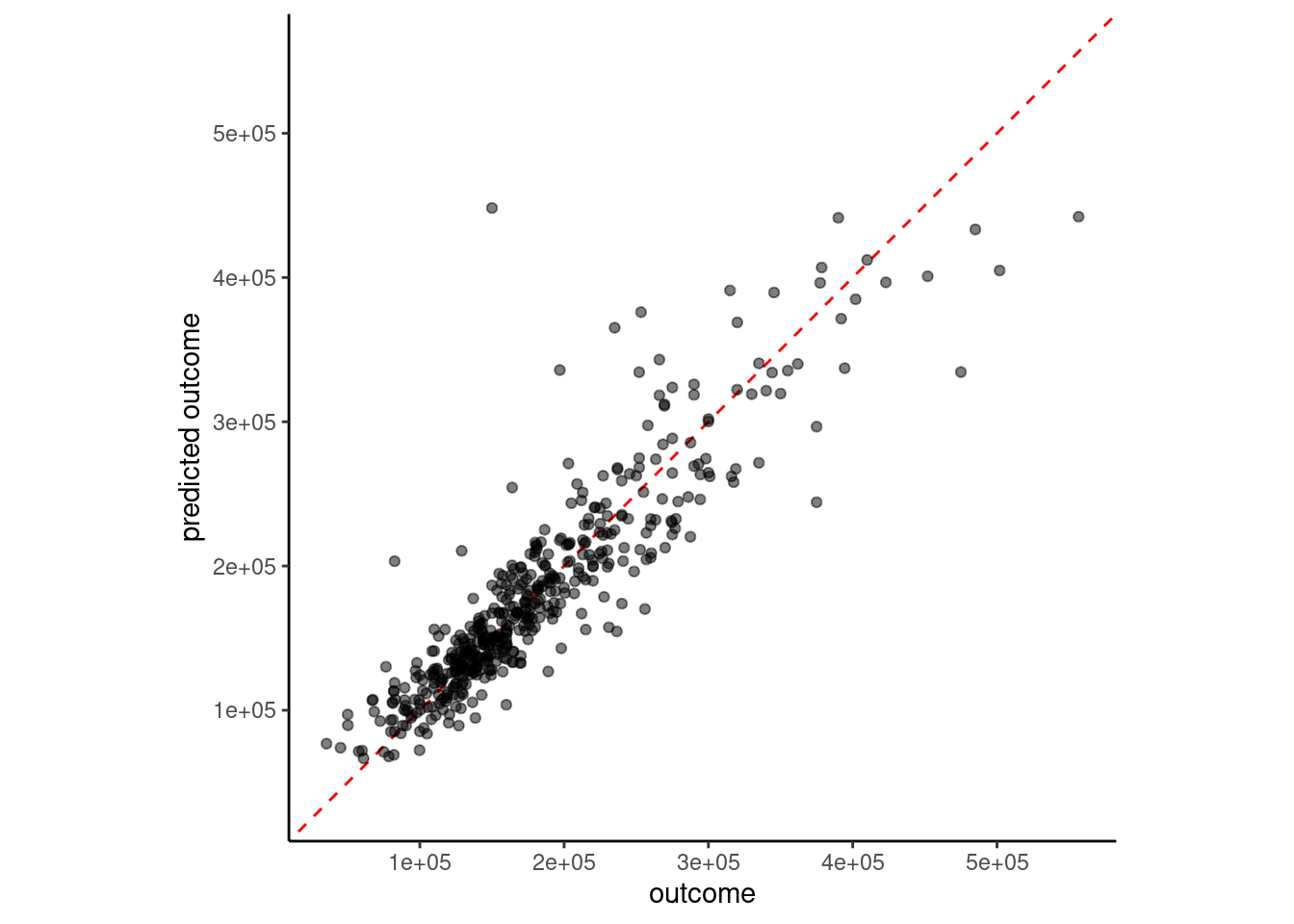

But 5NN may be overfit. k = 5 is pretty low

Again with k = 20

fit_20nn_5num <- 
  nearest_neighbor(neighbors = 20) |>   
  set_engine("kknn") |>   
  set_mode("regression") |> 
  fit(sale_price ~ ., data = feat_trn)

# A tibble: 9 × 2
  model                                  rmse_val
  <chr>                                     <dbl>
1 simple linear model                      51375.
2 4 feature linear model                   39903.
3 4 feature linear model with YJ           41660.
4 6 feature linear model w/ms_zoning       39846.
5 7 feature linear model                   34080.
6 8 feature linear model w/interaction     32720.
7 10 feature linear model w/interactions   32708.
8 5 numeric predictor 5nn                  32837.
9 5 numeric predictor 20nn                 30535.

That helped some

One more time with k = 50 to see where we are in the bias-variance function

fit_50nn_5num <- 
  nearest_neighbor(neighbors = 50) |>   
  set_engine("kknn") |>   
  set_mode("regression") |> 
  fit(sale_price ~ ., data = feat_trn)

# A tibble: 10 × 2
   model                                  rmse_val
   <chr>                                     <dbl>
 1 simple linear model                      51375.
 2 4 feature linear model                   39903.
 3 4 feature linear model with YJ           41660.
 4 6 feature linear model w/ms_zoning       39846.
 5 7 feature linear model                   34080.
 6 8 feature linear model w/interaction     32720.
 7 10 feature linear model w/interactions   32708.
 8 5 numeric predictor 5nn                  32837.
 9 5 numeric predictor 20nn                 30535.
10 5 numeric predictor 50nn                 31055.

Too high, now we have bias……
We will learn a more rigorous method for selecting the optimal value for $k$ (i.e., tuning this hyperparameter) in unit 5

To better understand bias-variance trade-off, let’s look at error across these three values of $k$ in train and validation for Ames

Training

Remember that training error would be 0 for k = 1
Training error is increasing as $k$ increases b/c it KNN is overfitting less (so its not fitting the noise in train as well)

rmse_vec(feat_trn$sale_price, 
         predict(fit_5nn_5num, feat_trn)$.pred)

[1] 19012.94

rmse_vec(feat_trn$sale_price, 
         predict(fit_20nn_5num, feat_trn)$.pred)

[1] 27662.2

rmse_vec(feat_trn$sale_price, 
         predict(fit_50nn_5num, feat_trn)$.pred)

[1] 31069.12

Validation

Validation error is first going down as $k$ increases (and it would have been very high for k = 1)
Bias is likely increasing a bit
But this is compensated by big decreases in overfitting variance
The trade-off is good for k = 20 relative to 5 and 1
At some point, as $k$ increases the increase in bias outweighed the decrease in variance and validation error increased too.

rmse_vec(feat_val$sale_price, 
         predict(fit_5nn_5num, feat_val)$.pred)

[1] 32837.37

rmse_vec(feat_val$sale_price, 
         predict(fit_20nn_5num, feat_val)$.pred)

[1] 30535.04

rmse_vec(feat_val$sale_price, 
         predict(fit_50nn_5num, feat_val)$.pred)

[1] 31054.6

Let’s do one final example and add one of our nominal variables into the model: ms_zoning

Need to collapse levels and then dummy

rec <- 
  recipe(sale_price ~ gr_liv_area + lot_area + year_built + garage_cars + 
           overall_qual + ms_zoning, data = data_trn) |> 
  step_impute_median(garage_cars) |> 
  step_mutate(overall_qual = as.numeric(overall_qual)) |> 
  step_mutate(ms_zoning = fct_collapse(ms_zoning,
                                 "residential" = c("res_high", "res_med", "res_low"),
                                 "commercial" = c("agri", "commer", "indus"),
                                 "floating" = "float")) |>
  step_dummy(ms_zoning) |> 
  step_scale(all_numeric_predictors())

prep, bake

rec_prep <- rec |> 
  prep(data_trn)

feat_trn <- rec_prep |> 
  bake(NULL)

feat_val <- rec_prep |> 
  bake(data_val)

fit_20nn_5num_mszone <- 
  nearest_neighbor(neighbors = 20) |>   
  set_engine("kknn") |>   
  set_mode("regression") |> 
  fit(sale_price ~ ., data = feat_trn)

evaluate

# A tibble: 11 × 2
   model                                   rmse_val
   <chr>                                      <dbl>
 1 simple linear model                       51375.
 2 4 feature linear model                    39903.
 3 4 feature linear model with YJ            41660.
 4 6 feature linear model w/ms_zoning        39846.
 5 7 feature linear model                    34080.
 6 8 feature linear model w/interaction      32720.
 7 10 feature linear model w/interactions    32708.
 8 5 numeric predictor 5nn                   32837.
 9 5 numeric predictor 20nn                  30535.
10 5 numeric predictor 50nn                  31055.
11 5 numeric predictor 20nn with ms_zoning   30172.

Now it helps.
Might have to do with interactions with other predictors that we didn’t model in the linear model
KNN automatically accommodates interactions. Why?
This model is a bit more complex and might benefit further from higher $k$

As a teaser, here is another performance metric for this model - $R^2$. Not too shabby! Remember, there is certainly some irreducible error in sale_price that will put a ceiling on $R^2$ and a floor on RMSE

rsq_vec(feat_val$sale_price, 
        predict(fit_20nn_5num_mszone, feat_val)$.pred)

[1] 0.8404044

Overall, we now have a model that predicts housing prices with about 30K of RMSE and accounting for 84% of the variance. I am sure you can improve on this!

3.10 Discussion

3.10.1 Announcements

Room change for two days
- Thursday, 2/15
- Thursday, 2/29
- Room 121
- If we like it……
Feedback - THANKS!
- consistent feedback will be implemented (as best I can!)
- captions
- vocabulary and concepts - new appendix
- use of web “book” - better thought of as lecture slides
- you can clone book_iaml. Render to slides with your notes, render to pdf
- Use of questions for dicussion
  - Didn’t work to read directly
  - Rank order based on frequency and importance
  - Put some in slack
  - Can’t do all. Ask in slack, ask in office hours or after discussion/lab
Reprex
- We need you to try to make reprex for help on application assignments
Homework is basically same for unit 4
- New dataset - titanic
- Do EDA but we don’t need to see it
- Fit KNN and RDA models (will learn about LDA, QDA and RDA in unit)
- Submit predictions. Free lunch!
- And for this free lunch….

read_csv(here::here(path_data, "lunch_003.csv")) |> 
  print_kbl()

Rows: 20 Columns: 2
── Column specification ────────────────────────────────────────────────────────
Delimiter: ","
chr (1): name
dbl (1): rmse_test

ℹ Use `spec()` to retrieve the full column specification for this data.
ℹ Specify the column types or set `show_col_types = FALSE` to quiet this message.

name	rmse_test
Dong	25495.53
Simental	28733.22
Phipps	28794.84
Yang	30420.01
Li	31534.42
Yu	31874.12
NA	32606.15
NA	33614.59
NA	33877.07
NA	33879.19
NA	34315.31
NA	34692.22
NA	35034.74
NA	35154.67
NA	35683.85
NA	36101.95
NA	36266.80
NA	36473.84
NA	38974.43
NA	42367.31

3.10.2 Sources of error

What are two broad sources of error?
What are two broad sources of reducible error. Describe what they are and factors that affect them?
Why do we need independent validation data to select the best model configuration?
Why do we need test data if we used validation data to select among many model configurations
What is RMSE? Connect it to metric you already know? How is it being used in lm (two ways)?; in knn (one way)?
How does bias and variance manifest when you look at your performance metric (RMSE) in training and validation sets?
Will the addition of new features to a (lm?) model always reduce RMSE in train? in validation? Connect to concepts of bias and variance

3.10.3 KNN

How does KNN use training data to make predictions
What is k and how does it get used when making predictions?
What is the impact of k on bias and variance/overfitting?
k=1: performance in train? in val?
Distance measures: use Euclidean (default in kknn)!
Tuning K: stay “tuned”

3.10.4 Interaction in KNN - Consider bias first (but also variance) in this example

Simulate data
Fit models for lm and knn with and without interaction
Took some shortcuts (no recipe, predict back into train)

n <- 200
set.seed(5433)

d <- tibble(x1 = runif(n, 0,100), # uniform
               x2 = rep(c(0,1), n/2), # dichotomous
               x1_x2 = x1*x2, # interaction
               y = rnorm(n, 0 + 1*x1 + 10*x2 + 10* x1_x2, 20)) #DGP + noise

fit_lm <- 
  linear_reg() |>   
  set_engine("lm") |>   
  fit(y ~ x1 + x2, data = d)

fit_lm_int <- 
  linear_reg() |>   
  set_engine("lm") |>   
  fit(y ~ x1 + x2 + x1_x2, data = d)

fit_knn <- 
  nearest_neighbor(neighbors = 20) |>   
  set_engine("kknn") |>   
  set_mode("regression") |> 
  fit(y ~ x1 + x2, data = d)

fit_knn_int <- 
  nearest_neighbor(neighbors = 20) |>   
  set_engine("kknn") |>   
  set_mode("regression") |> 
  fit(y ~ x1 + x2 + x1_x2, data = d)

d <- d |> 
  mutate(pred_lm = predict(fit_lm, d)$.pred,
         pred_lm_int = predict(fit_lm_int, d)$.pred,
         pred_knn = predict(fit_knn, d)$.pred,
         pred_knn_int = predict(fit_knn_int, d)$.pred)

Predictions from linear model with and without interaction
- You NEED interaction features with LM

d |> 
  ggplot(aes(x = x1, group = factor(x2), color = factor(x2))) +
    geom_line(aes(y = pred_lm)) +
    geom_point(aes(y = y)) +
    ggtitle("lm without interaction") +
    ylab("y") +
    scale_color_discrete(name = "x2")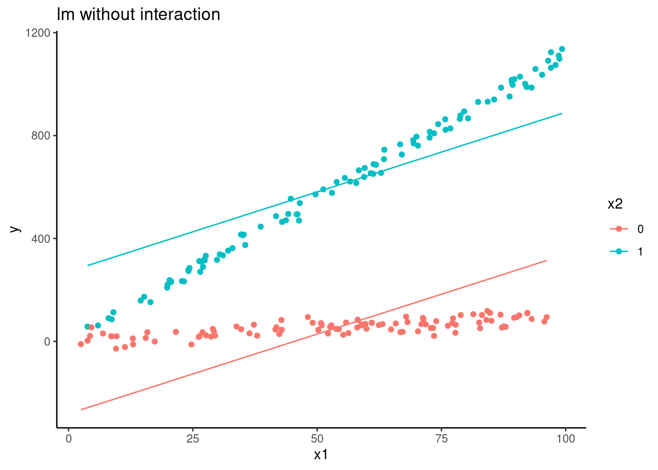

d |> 
  ggplot(aes(x = x1, group = factor(x2), color = factor(x2))) +
    geom_line(aes(y = pred_lm_int)) +
    geom_point(aes(y = y)) +
    ggtitle("lm with interaction") +
    ylab("y") +
    scale_color_discrete(name = "x2")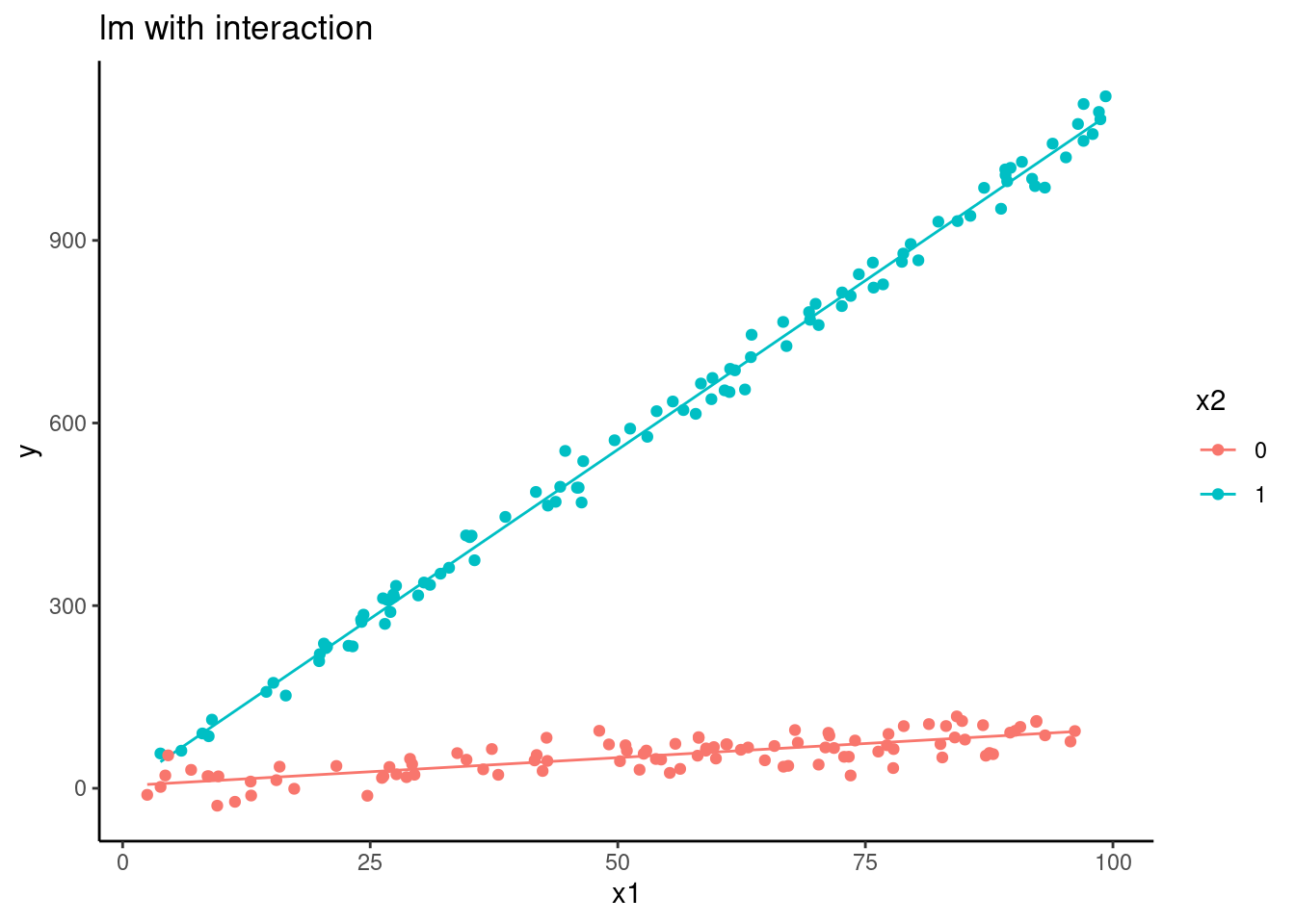

Predictions from KNN with and without interaction
- You do NOT need interaction features with KNN!

d |> 
  ggplot(aes(x = x1, group = factor(x2), color = factor(x2))) +
    geom_line(aes(y = pred_knn)) +
    geom_point(aes(y = y)) +
    ggtitle("KNN without interaction") +
    ylab("y") +
    scale_color_discrete(name = "x2")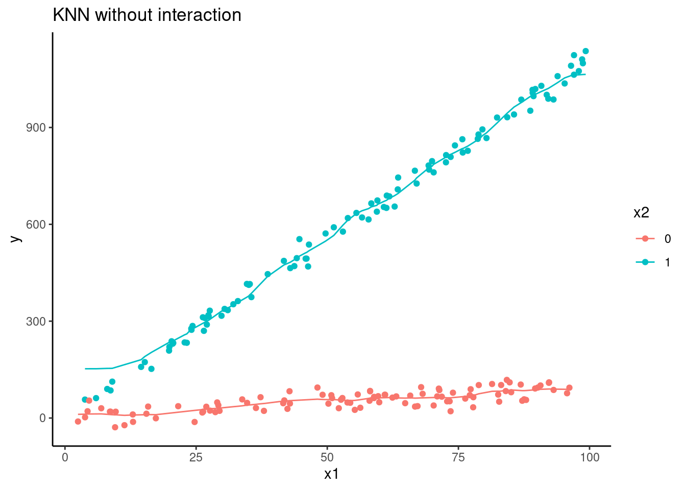

d |> 
  ggplot(aes(x = x1, group = factor(x2), color = factor(x2))) +
    geom_line(aes(y = pred_knn_int)) +
    geom_point(aes(y = y)) +
    ggtitle("KNN with interaction") +
    ylab("y") +
    scale_color_discrete(name = "x2")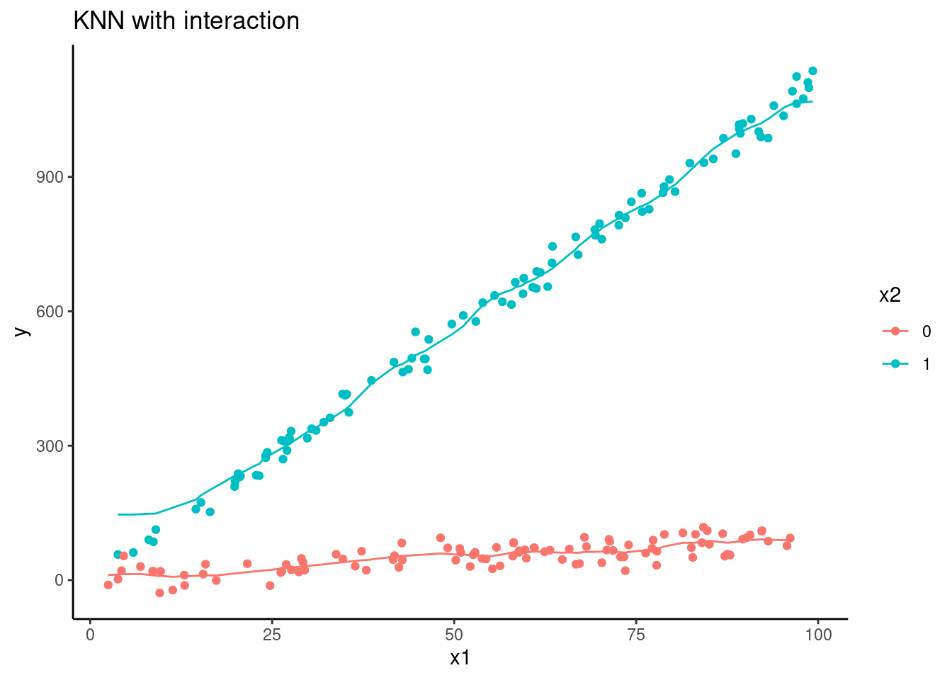

3.10.5 LM vs. KNN better with some predictors or overall?

“Why do some features seem to improve performance more in linear models or only in KNNs?”
“What are some contexts where KNN doesn’t work well? In other words, what are the advantages/disadvantages of using KNN?”
- Always comes down to bias vs. variance
- Flexibility and N are key moderators of these two key factors.
- k? - impact on bias, variance?
KNN for explanation?
- Visualizations (think of interaction plot above) make clear the effect
- Will learn more (better visualizations, variable importance, model comparisons) in later unit

3.10.6 Normalizing transformations - Yeo Johnson

when needed for lm?
when needed for knn?

3.10.7 Dummy coding

Why do we do it?
Describe the values assigned to the dummy coded features
Why these values? In other words, how can you interpret the effect of a dummy coded feature?
How is it different from one-hot coding. When to use or not use one-hot coding?

3.10.8 Exploration

“I feel that I can come up with models that decrease the RMSE, but I don’t have good priors on whether adding any particular variable or observation will result in an improved model. I still feel a little weird just adding and dropping variables into a KNN and seeing what gets the validation RMSE the lowest (even though because we’re using validation techniques it’s a fine technique)”
- Exploration is learning. This is research. If you knew the answer you wouldn’t be doing the study
- Domain knowledge is still VERY important
- Some algorithms (LASSO, glmnet) will help with feature selection
- staying organized
  - Script structure
  - Good documentation - QMD as analysis notebook
- Some overfitting to validation will occur? Consequence? Solutions?

3.10.9 “Curse of dimensionality” - Bias vs. variance

Missing features produce biased models.
Unnecessary features or even many features relative to N produce variance
Does your available N in your algorithm support the features you need to have low bias.
- Mostly an empirical question - can’t really tell otherwise outside of simulated data. Validation set is critical!
- Flexible models often need more N holding features constant
- Regularization (unit 6) will work well when lots of features

3.10.10 Transformations of numeric predictors

Use of plot_truth() [predicted vs. observed]
Residuals do not have mean of 0 for every $\hat{y}$
- Consequence: biased parameter estimates. Linear is bad DGP
- Also bad test of questions RE the predictor (underestimate? misinform)
Non-normal residuals
- Consequence: lm parameter estimates still unbiased (for linear DGP) but more “efficient” solutions exist
- Bad for prediction b/c higher variance than other solutions
- May suggest omission of variables
Heteroscasticity
- Consequence: Inefficient and inaccurate standard errors.
- Statistical tests wrong
- Poor prediction for some (where larger variance of residuals) $\hat{y}$
- higher variance overall than other solutions - bad again for prediction
Transformation of outcome?
- metric
- back to raw predictions

3.10.11 “In GLM, why correlation/collinearity among predictors will cause larger variance? Is it because of overfitting?”

3.10.12 KNN (black box) for explanatory purposes

James, Gareth, Daniela Witten, Trevor Hastie, and Robert Tibshirani. 2023. An Introduction to Statistical Learning: With Applications in R. 2nd ed. Springer Texts in Statistics. New York: Springer-Verlag.