library(keras, exclude = "get_weights")
library(magrittr, exclude = c("set_names", "extract"))10 Advanced Models: Neural Networks
10.1 Overview of Unit
10.1.1 Learning Objectives
- What are neural networks
- Types of neural networks
- Neural network architecture
- layers and units
- weights and biases
- activation functions
- cost functions
- optimization
- epochs
- batches
- learning rate
- How to fit 3 layer MLPs in tidymodels using Keras
10.1.2 Readings
Post questions to the readings channel in Slack
10.1.3 Lecture Videos
- Lecture 1: But what is a Neural Network? ~ 19 mins
- Lecture 2: Gradient descent, how neural networks learn ~ 21 mins
- Lecture 3: What is backpropagation really doing? ~ 13 mins
- Optional Lecture 4: Backpropagation calculus ~ 10 mins
- Lecture 5: Introduction and the MNIST dataset ~ 14 mins
- Lecture 6: Fitting neural networks in tidymodels with Keras ~ 18 mins
- Lecture 7: Addressing overfitting - Intro and L2 ~ 5 mins
- Lecture 8: Addressing overfitting - Dropout ~ 4 mins
- Lecture 9: Addressing overfitting - Early stopping ~ 8 mins
- Lecture 10: Selecting model configurations and final remarks ~ 8 mins
Post questions to the video-lectures channel in Slack
10.1.4 Coding Assignment
Post questions to application-assignments Slack channel
Submit the application assignment here and complete the unit quiz by 8 pm on Wednesday, April 3rd
10.2 Introduction to Nerual Networks with Keras in R
We will be using the keras engine to fit our neural networks in R.
The keras package provides an R Interface to the Keras API in Python.
From the website:
Keras is a high-level neural networks API developed with a focus on enabling fast experimentation. Being able to go from idea to result with the least possible delay is key to doing good research.
Keras has the following key features:
- Allows the same code to run on CPU or on GPU, seamlessly.
- User-friendly API - which makes it easy to quickly prototype deep learning models.
- Built-in support for basic multi-layer perceptrons, convolutional networks (for computer vision), recurrent networks (for sequence processing), and any combination of both.
- Supports arbitrary network architectures: multi-input or multi-output models, layer sharing, model sharing, etc. This means that Keras is appropriate for building essentially any deep learning model, from a memory network to a neural Turing machine.
Keras is actually a wrapper around an even more extensive open source platform, TensorFlow, which has also been ported to the R environment
TensorFlow is an end-to-end open source platform for machine learning. It has a comprehensive, flexible ecosystem of tools, libraries and community resources that lets researchers push the state-of-the-art in ML and developers easily build and deploy ML powered applications.
TensorFlow was originally developed by researchers and engineers working on the Google Brain Team within Google’s Machine Intelligence research organization for the purposes of conducting machine learning and deep neural networks research
If you are serious about focusing primarily or exclusively on neural networks, you will probably work directly within Keras in R or Python. However, tidymodels gives us access to 3 layer (single hidden layer) MLP neural networks through the keras engine. This allows us to fit simple (but still powerful) neural networks using all the tools (and code/syntax) that you already know. Yay!
If you plan to use Keras directly in R, you might start with this book. I’ve actually found it useful even in thinking about how to interface with Keras through tidymodels.
Getting tidymodels configured to use the keras engine can take a little bit of upfront effort.
We provide an appendix to guide you through this process
If you havent already set this up, please do so immediately so that you can reach out to us for support if you need it
Once you have completed this one-time installation, you can now use the keras engine through tidymodels like any other engine. No need to do anything different from your normal tidymodeling workflow.
You should also know that Keras is configured to use GPUs rather than CPU (GPUs allow for highly parallel fitting of neural networks).
- However, it works fine with just a CPU as well.
- It will generate some errors to tell you that you aren’t set up with a GPU (and then it will tell you to ignore those error messages).
- This is an instance where you can ignore the messages!
10.3 Setting up our Environment
Now lets start fresh
- We load our normal environment including source files, parallel processing and cache support if we plan to use it (code not displayed)
- keras will work with R without loading it or other packages (beyond what we always load). However, there will be some function conflicts.
- So we will load keras and exclude the conflict
- We also need to load magrittr and exclude two of its conflicting functions
10.4 The MNIST dataset
The MNIST database (Modified National Institute of Standards and Technology database) is a large database of handwritten digits that is commonly used for training and testing in the field of machine learning.
It consists of two sets:
- There are 60,000 images from 250 people in train
- There are 10,000 images from a different 250 people in test (from different people than in train)
Each observation in the datasets represent a single image and its label
- Each image is a 28 X 28 grid of pixels = 784 predictors (x1 - x784)
- Each label is the actual value (0-9; y). We will treat it as categorical because we are trying to identify each number “category”, predicting a label of “4” when the image is a “5” is just as bad as predicting “9”
Let’s start by reading train and test sets
data_trn <- read_csv(here::here(path_data, "mnist_train.csv.gz"),
                     col_types = cols()) |>
  mutate(y = factor(y, levels = 0:9, labels = 0:9))
data_trn |> dim()
[1] 60000 785data_test <- read_csv(here::here(path_data, "mnist_test.csv"),
col_types = cols()) |>
mutate(y = factor(y, levels = 0:9, labels = 0:9))
data_test |> dim()[1] 10000 785Here is some very basic info on the outcome distribution
- in train
data_trn |> tab(y)# A tibble: 10 × 3
y n prop
<fct> <int> <dbl>
1 0 5923 0.0987
2 1 6742 0.112
3 2 5958 0.0993
4 3 6131 0.102
5 4 5842 0.0974
6 5 5421 0.0904
7 6 5918 0.0986
8 7 6265 0.104
9 8 5851 0.0975
10 9 5949 0.0992data_trn |> plot_bar("y")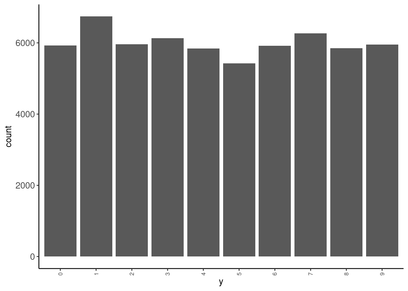
- in test
data_test|> tab(y)# A tibble: 10 × 3
y n prop
<fct> <int> <dbl>
1 0 980 0.098
2 1 1135 0.114
3 2 1032 0.103
4 3 1010 0.101
5 4 982 0.0982
6 5 892 0.0892
7 6 958 0.0958
8 7 1028 0.103
9 8 974 0.0974
10 9 1009 0.101 data_test |> plot_bar("y")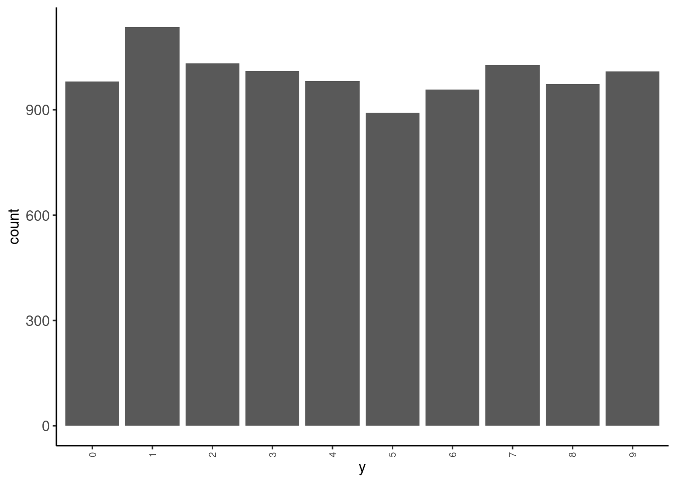
Let’s look at some of the images. We will need a function to display these images. We will use as.cimg() from the imager package
display_image <- function(data){
  message("Displaying: ", data$y)

  data |>
    select(-y) |>
    unlist(use.names = FALSE) |>
    imager::as.cimg(x = 28, y = 28) |>
    plot(axes = FALSE)
}
Observations 1, 3, 10, and 100 in training set
data_trn |>
  slice(1) |>
  display_image()
Displaying: 5
data_trn |>
  slice(3) |>
  display_image()
Displaying: 4
data_trn |>
  slice(10) |>
  display_image()
Displaying: 4
data_trn |>
  slice(100) |>
  display_image()
Displaying: 1
And here is the first observation in test set
data_test |>
  slice(1) |>
  display_image()
Displaying: 7
Let’s understand the individual predictors a bit more
- Each predictor is a pixel in the 28 X 28 grid for the image
- Pixel intensity is coded for intensity in the range from 0 (black) to 255 (white)
- First 28 variables are the top row of 28 pixels
- Next 28 variables are the second row of 28 pixels
- There are 28 rows of 28 predictors total (784 predictors)
- Lets understand this by changing values for individual predictors
- Here is the third image again
What will happen to the image if I change the value of predictor x25 to 255
data_trn |>
  slice(3) |>
  display_image()
Displaying: 4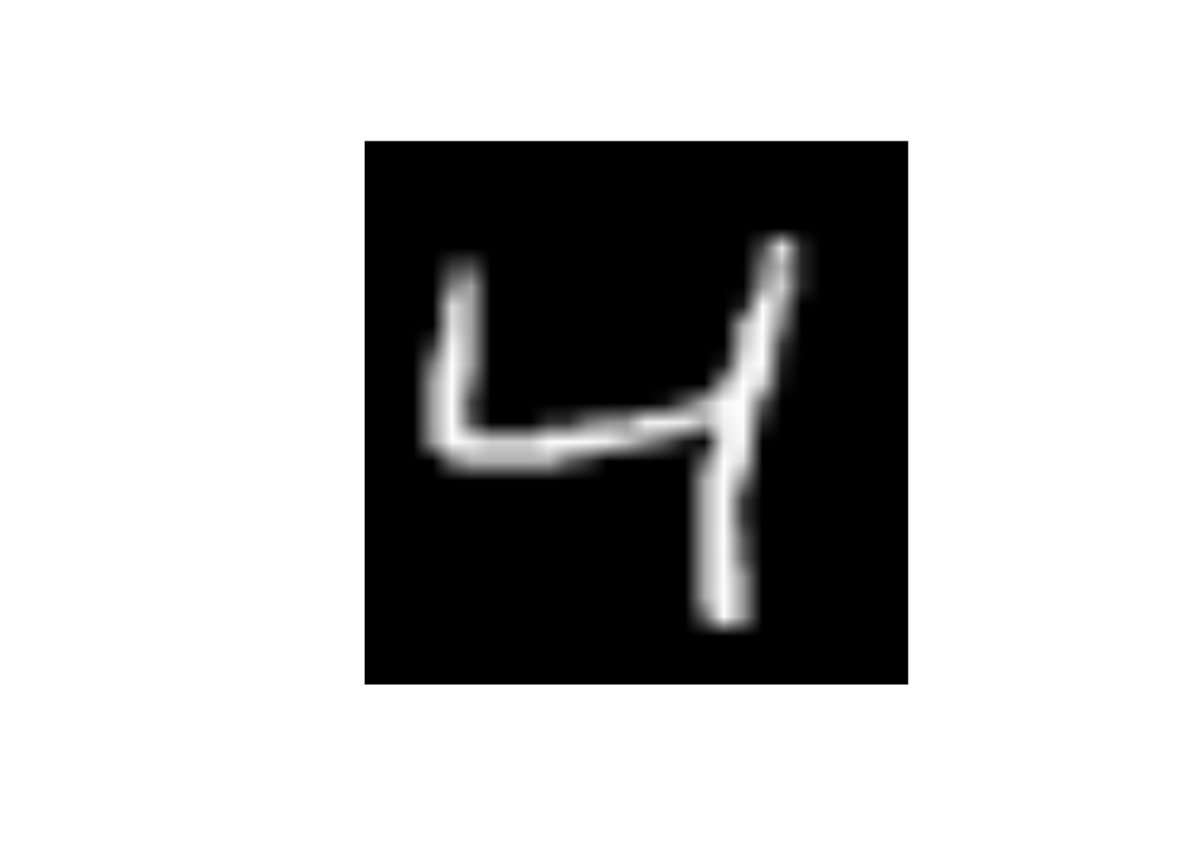
- Change the
x25to 255
data_trn |>
  slice(3) |>
  mutate(x25 = 255) |>
  display_image()
Displaying: 4
What will happen to the image if I change the value of predictor x29 to 255
- Change the
x29to 255
data_trn |>
  slice(3) |>
  mutate(x29 = 255) |>
  display_image()
Displaying: 4
What will happen to the image if I change the value of predictor x784 to 255
- Change the
x784to 255
data_trn |>
  slice(3) |>
  mutate(x784 = 255) |>
  display_image()
Displaying: 4
10.5 Fitting Neural Networks
Let’s train some models to understand some basics about neural networks and the use of Keras within tidymodels
We will fit some configurations in the full training set and evaluate their performance in test
We are NOT using test to select among configurations (it wouldn’t be a true test set then) but only for instructional purposes.
We will start with an absolute minimal recipe and mostly defaults for the statistical algorithm
We will build up to more complex (and better) configurations
We will end with a demonstration of the use of the single validation set approach to select among model configurations
Let’s start with a minimal recipe
- 10 level categorical outcome as factor
- Will be used to establish 10 output neurons
rec_min <-
  recipe(y ~ ., data = data_trn)
Here are feature matrices for train and test using this recipe
rec_min_prep <- rec_min |>
  prep(data_trn)

feat_trn <- rec_min_prep |>
  bake(NULL)

feat_test <-rec_min_prep |>
  bake(data_test)
And let’s use a mostly out of the box (defaults) 3 layer (1 hidden layer) using Keras engine
Defaults:
- hidden units = 5
- penalty = 0
- dropout = 0
- activation = “softmax” for hidden units layer
- epochs = 20
- seeds = sample.int(10^5, size = 3)
The default activation for the hidden units when using Keras through tidymodels is softmax not sigmoid as per the basic models discussed in the book and lectures.
- The activation for the output layer will always be
softmaxfor classification problems when using Keras through tidymodels- This is likely a good choice
- It provides scores that function like probabilities for each categorical response
- The activation for the output layer will always be ‘linear’ for regression problems.
- Also a generally good choice
- The hidden units can have a variety of different activation functions
linear,softmax,relu, andeluthrough tidymodels- Additional activation functions (and many other “dials”) are available in Keras directly
We will adjust seeds from the start
There are a number of points in the fitting process where random numbers needed by Keras
- initializing weights for hidden and output layers
- selecting units for
dropout - selecting batches within epochs
tidymodels lets us provide three seeds to make the first two bullet points more reproducible.
There seems to still be some randomness across runs due to batch selection (and possibly other opaque steps)
set.seed(1234567)
fit_seeds <- sample.int(10^5, size = 3)  # c(87591, 536, 27860)
We will also set verbose = 0 for now
- This turns off messages and plots about epoch level performance
- At this point, verbose would only report performance in the training data, which isn’t that informative
- We will turn it on later when we learn how to get performance in a validation set
- Nonetheless, you might still turn it on if you just want feedback on how long it will take for the fit to complete.
Let’s fit this first model configuration in training set
verbose = 0seeds = fit_seeds
fit_1 <-
    mlp() |>
    set_mode("classification") |>
    set_engine("keras",
               verbose = 0,
               seeds = fit_seeds) |>
    fit(y ~ ., data = feat_trn)
NOTE: The first model fit with Keras in each new session will generate those warnings/errors about GPU. You can ignore them.
Here is this model’s performance in test
It’s not that great (What would you expect by chance?)
accuracy_vec(feat_test$y, predict(fit_1, feat_test)$.pred_class)313/313 - 1s - 529ms/epoch - 2ms/step[1] 0.2063Theoretically, the scale of the inputs should not matter
HOWEVER, gradient descent works better with inputs on the same scale
We will also want inputs with the same variance if we later apply L2 regularization to our models
- There is a lot of discussion about how best to scale inputs
- Best if the input means are near zero
- Best if variances are comparable
We could:
- Use
step_normalize()[Bad choice of function names by tidymodel folks; standardize vs. normalize] - Use
step_range() - Book range corrected based on known true range (
/ 255)
We will usestep_normalize()
rec_scaled_wrong <-
  recipe(y ~ ., data = data_trn) |>
  step_normalize(all_predictors())
This is wrong! Luckily we glimpsed our feature matrix (not displayed here)
For example
data_trn$x1 |> sd()[1] 0Let’s remove zero variance predictors before we scale
- To be clear, zero variance features are NOT a problem for neural networks (though clearly they won’t help either).
- But they WILL definitely cause problems for some scaling transformations.
rec_scaled <-
  recipe(y ~ ., data = data_trn) |>
  step_zv(all_predictors()) |>
  step_normalize(all_predictors())
We now have 717 (+ y) features rather than 28 * 28 = 784 features
rec_scaled_prep <- rec_scaled |>
  prep(data_trn)

feat_trn <- rec_scaled_prep |>
  bake(NULL)

dim(feat_trn)
[1] 60000 718Let’s also make the feature matrix for test. This will exclude features that were zero variance in train and scale them by their mean and sd in train
feat_test <- rec_scaled_prep |>
  bake(data_test)

dim(feat_test)
[1] 10000 718Let’s fit and evaluate this new feature set with no other changes to the model configuration
fit_2 <-
  mlp() |>
  set_mode("classification") |>
  set_engine("keras", verbose = 0, seeds = fit_seeds) |>
fit(y ~ ., data = feat_trn)- That helped a LOT
- Still could be better though (but it always impresses me! ;-)
accuracy_vec(feat_test$y, predict(fit_2, feat_test)$.pred_class)313/313 - 1s - 513ms/epoch - 2ms/step[1] 0.4958There are many other recommendations about feature engineering to improve the inputs
These include:
- Normalize (and here I mean true normalization; e.g.,
step_BoxCox(),step_YeoJohnson()) - De-correlate (e.g.,
step_pca()but retain all features?)
You can see some discussion of these issues here and here to get you started. The paper linked in the stack overflow response is also a useful starting point.
Some preliminary modeling EDA on my part suggested these additional considerations didn’t have major impact on the performance of our models with this dataset so we will stick with just scaling the features.
It is not surprising that a model configuration with only one hidden layer and 5 units isn’t sufficient for this complex task
Let’s try 30 units (cheating based on the book chapter!! ;-)
fit_5units <- mlp(hidden_units = 30) |>
    set_mode("classification") |>
    set_engine("keras", verbose = 0, seeds = fit_seeds) |>
fit(y ~ ., data = feat_trn)- Bingo! Much, much better!
- We could see if even more units works better still but I won’t follow that through here for sake of simplicity
accuracy_vec(feat_test$y, predict(fit_5units, feat_test)$.pred_class)313/313 - 1s - 554ms/epoch - 2ms/step[1] 0.9386The Three Blue 1 Brown videos had a brief discussion of the relu activation function.
Let’s see how to use other activation functions and if this one helps.
fit_relu <- mlp(hidden_units = 30, activation = "relu") |>
  set_mode("classification") |>
  set_engine("keras", verbose = 0, seeds = fit_seeds) |>
fit(y ~ ., data = feat_trn)accuracy_vec(feat_test$y, predict(fit_relu, feat_test)$.pred_class)313/313 - 0s - 414ms/epoch - 1ms/step[1] 0.964710.6 Dealing with Overfitting
As you might imagine, given the number of weights to be fit in even a modest neural network (our 30 hidden unit network has 21,850 parameters to estimate), it is easy to become overfit
- 21,540 for hidden layer (717 * 30 weight + 30 biases)
- 310 for output layer (30 * 10 weights, + 10 biases)
fit_reluparsnip model object
Model: "sequential_3"
________________________________________________________________________________
Layer (type) Output Shape Param #
================================================================================
dense_6 (Dense) (None, 30) 21540
dense_7 (Dense) (None, 10) 310
================================================================================
Total params: 21850 (85.35 KB)
Trainable params: 21850 (85.35 KB)
Non-trainable params: 0 (0.00 Byte)
________________________________________________________________________________This will be an even bigger problem if you aren’t using “big” data
There are a number of different methods available to reduce potential overfitting
- Simplify the network architecture (fewer units, fewer layers)
- L2 regularization
- Dropout
- Early stopping or monitoring validation error to prevent too many epochs
10.6.1 Regularization or Weight Decay
L2 regularization is implemented in essentially the same fashion as you have seen it previously (e.g., glmnet)
The cost function is expanded to include a penalty based on the sum of the squared weights multiplied by \(\lambda\).
In the tidymodels implementation of Keras:
\(\lambda\) is called
penaltyand is set and/or (ideally) tuned via thepenaltyargument inmlp()Common values for the L2
penaltyto tune a neural network are often on a logarithmic scale between 0 and 0.1, such as 0.1, 0.001, 0.0001, etc.penalty = 0(the default) means no L2 regularizationKeras implements other penalties (L1, and a mixture) but not currently through tidymodels
Here is a starting point for more reading on regularization in neural networks
Let’s set penalty = .0001.
fit_penalty <- mlp(hidden_units = 30, activation = "relu", penalty = .0001) |>
  set_mode("classification") |>
  set_engine("keras", verbose = 0, seeds = fit_seeds) |>
fit(y ~ ., data = feat_trn)- Looks like there is not much benefit to regularization for this network.
- Would likely provide much greater benefit in smaller N contexts or with more complicated model architectures (more hidden units, more hidden unit layers).
accuracy_vec(feat_test$y, predict(fit_penalty, feat_test)$.pred_class)313/313 - 0s - 355ms/epoch - 1ms/step[1] 0.966110.6.2 Dropout
Dropout is a second technique to minimize overfitting.
Here is a clear description of dropout from a blog post on the Machine Learning Mastery:
Dropout is a technique where randomly selected neurons are ignored during training. They are “dropped-out” randomly. This means that their contribution to the activation of downstream neurons is temporally removed on the forward pass and any weight updates are not applied to the neuron on the backward pass.
As a neural network learns, neuron weights settle into their context within the network. Weights of neurons are tuned for specific features providing some specialization. Neighboring neurons come to rely on this specialization, which if taken too far can result in a fragile model too specialized to the training data.
You can imagine that if neurons are randomly dropped out of the network during training, that other neurons will have to step in and handle the representation required to make predictions for the missing neurons. This is believed to result in multiple independent internal representations being learned by the network.
The effect is that the network becomes less sensitive to the specific weights of neurons. This in turn results in a network that is capable of better generalization and is less likely to overfit the training data.
For further reading, you might start with the 2014 paper by Srivastava, et al that proposed the technique.
In tidymodels, you can set or tune the amount of dropout via the dropout argument in mlp()
- Srivastava, et al suggest starting with values around .5.
- You might consider a range between .1 and .5
droppout = 0(the default) means no dropout- In tidymodels implementation of Keras, you can use a non-zero
penaltyordropoutbut not both
Let’s try dropout = .1.
fit_dropout <- mlp(hidden_units = 30, activation = "relu", dropout = .1) |>
  set_mode("classification") |>
  set_engine("keras", verbose = 0, seeds = fit_seeds) |>
fit(y ~ ., data = feat_trn)- Looks like there may be a little benefit but not substantial.
- Would likely provide much greater benefit in smaller N contexts or with more complicated model architectures (more hidden units, more hidden unit layers).
accuracy_vec(feat_test$y, predict(fit_dropout, feat_test)$.pred_class)313/313 - 1s - 515ms/epoch - 2ms/step[1] 0.965310.6.3 Number of Epochs and Early Stopping
Now that we have a model that is working well, lets return to the issue of number of epochs
- Too many epochs can lead to overfitting
- Too many epochs also just slow things down (not a bit deal if using GPU or overnight but still…..)
- Too few epochs can lead to under-fitting (which also produces poor performance)
- The default of
epochs = 20is a reasonable starting point for a network with one hidden layer but may not work for all situations
Monitoring training error (loss, accuracy) is not ideal b/c it will tend to always decrease
- This is what you would get if you set
verbose = 1
Validation error is what you need to monitor
- Validation error will increase when the model becomes overfit to training
- We can have Keras hold back some portion of the training data for validation
validation_split = 1/6- We pass it in as an optional argument in
set_engine() - We can use this to monitor validation error rather than training error by epoch.
- You can fit an exploratory model with
epochs = 50to review the plot - This can allow us to determine an appropriate value for
epochs
Let’s see this in action in the best model configuration without regularization or dropout
NOTE:
epochs = 50verbose = 1metrics = c("accuracy")validation_split = 1/6- You will see message updates and a plot that tracks training and validation loss and accuracy across epochs
- This is not rendered into my slides but the plot and messages are pretty clear
- You can use this information to choose appropriate values for
epoch val_accuracyhad plateau andval_losshad started to creep up by 10 epochs.
fit_epochs50 <- mlp(hidden_units = 30, activation = "relu", epochs = 50) |>
  set_mode("classification") |>
  set_engine("keras", verbose = 1, seeds = fit_seeds,
             metrics = c("accuracy"),
             validation_split = 1/6) |>
  fit(y ~ ., data = feat_trn)
In some instances, it may be that we want to do more than simply look at epoch performance plots during modeling EDA
We can instead set the number of epochs to be high but use an early stopping callback to end the training early at an optimal time
Callbacks allow us to interrupt training.
- There are many types of callbacks in Keras
- We will only discuss
callback_early_stopping() - We set up callbacks in a list
- We pass them in as an optional argument in
set_engine()usingcallbacks = - Notice the arguments for
callback_early_stopping() - We also must provide validation error. Here we set
validation_split = 1/6 - This is a method to tune or select best number of epochs.
- I haven’t yet figured out where the epochs at termination are saved so need to watch the feedback. It was 35 epochs here
- As always, we could next refit to the full training set after we have determined the optimal number of epochs. We won’t do that here.
This fit stopped at 15 epochs
callback_list <- list(keras::callback_early_stopping(monitor = "val_loss",
                                                     min_delta = 0,
                                                     patience = 10))
fit_early <- mlp(hidden_units = 30, activation = "relu", epochs = 200) |>
set_mode("classification") |>
set_engine("keras", verbose = 1,
seeds = fit_seeds,
metrics = c("accuracy" ),
validation_split = 1/6,
callbacks = callback_list) |>
fit(y ~ ., data = feat_trn)accuracy_vec(feat_test$y, predict(fit_early, feat_test)$.pred_class)313/313 - 0s - 430ms/epoch - 1ms/step[1] 0.9642Coding sidebar: You can see many of the optional arguments you can set for Keras in the help here.
And you can see more info about callback_early_stopping() here
10.7 Using Resampling to Select Best Model Configuration
Developing a good network artchitecture and considering feature enginnering options involves experimentation
- This is what Keras is designed to do
- tidymodels allows this too
- We need to evaluate configurations with a valid method to evaluate performance
- validation split metric
- k-fold metric
- bootstrap method
- Each can be paired with
fit_resamples()ortune_grid()
- We need to be systematic
tune_grid()helps with this too- recipes can be tuned as well (outside the scope of this course)
Here is an example where we can select among many model configurations that differ across multiple network characteristics
- Evaluate with validation split accuracy
- Sample size is relatively big so we have 10,000 validation set observations. Should offer a low variance performance estimate
- K-fold and bootstrap would still be better but big computation costs (too big for this web book but could be done in real life!)
Its really just our normal workflow at this point
- Get splits (validation splits in this example)
set.seed(102030)
splits_validation <-
  data_trn |>
validation_split(prop = 5/6)- Set up grid of hyperparameter values
grid_keras <- expand_grid(hidden_units = c(5, 10, 20, 30, 50, 100),
penalty = c(.00001, .0001, .01, .1))- Use
tune_grid()to fit models in training and predict into validation set for each combination of hyperparameter values
fits_nn <- cache_rds(
  expr = {
    mlp(hidden_units = tune(), penalty = tune(), activation = "relu") |>
    set_mode("classification") |>
    # setting to verbose = 1 to track progress.  Training error not that useful
    set_engine("keras", verbose = 1, seeds = fit_seeds) |>
    tune_grid(preprocessor = rec_scaled,
                  grid = grid_keras,
                  resamples = splits_validation,
                  metrics = metric_set(accuracy))
  },
  rerun = rerun_setting,
  dir = "cache/010/",
file = "fits_nn")- Find model configuration with best performance in the held-out validation set
show_best(fits_nn)# A tibble: 5 × 8
hidden_units penalty .metric .estimator mean n std_err
<dbl> <dbl> <chr> <chr> <dbl> <int> <dbl>
1 100 0.00001 accuracy multiclass 0.973 1 NA
2 100 0.0001 accuracy multiclass 0.970 1 NA
3 50 0.0001 accuracy multiclass 0.967 1 NA
4 50 0.00001 accuracy multiclass 0.966 1 NA
5 30 0.00001 accuracy multiclass 0.962 1 NA
.config
<chr>
1 Preprocessor1_Model21
2 Preprocessor1_Model22
3 Preprocessor1_Model18
4 Preprocessor1_Model17
5 Preprocessor1_Model1310.8 Other Details
We can get a better sense of how tidymodels is interacting with Keras by looking at the function that is called
mlp(hidden_units = 30, activation = "relu", dropout = .1) |>
  set_mode("classification") |>
  set_engine("keras", verbose = 0, seeds = fit_seeds) |>
  translate()
Single Layer Neural Network Model Specification (classification)
Main Arguments:
hidden_units = 30
dropout = 0.1
activation = relu
Engine-Specific Arguments:
verbose = 0
seeds = fit_seeds
Computational engine: keras
Model fit template:
parsnip::keras_mlp(x = missing_arg(), y = missing_arg(), hidden_units = 30,
dropout = 0.1, activation = "relu", verbose = 0, seeds = fit_seeds)keras_mlp() is a wrapper around the calls to Keras. Lets see what it does
keras_mlpfunction (x, y, hidden_units = 5, penalty = 0, dropout = 0, epochs = 20,
activation = "softmax", seeds = sample.int(10^5, size = 3),
...)
{
if (penalty > 0 & dropout > 0) {
rlang::abort("Please use either dropoput or weight decay.",
call. = FALSE)
}
if (!is.matrix(x)) {
x <- as.matrix(x)
}
if (is.character(y)) {
y <- as.factor(y)
}
factor_y <- is.factor(y)
if (factor_y) {
y <- class2ind(y)
}
else {
if (isTRUE(ncol(y) > 1)) {
y <- as.matrix(y)
}
else {
y <- matrix(y, ncol = 1)
}
}
model <- keras::keras_model_sequential()
if (penalty > 0) {
model %>% keras::layer_dense(units = hidden_units, activation = activation,
input_shape = ncol(x), kernel_regularizer = keras::regularizer_l2(penalty),
kernel_initializer = keras::initializer_glorot_uniform(seed = seeds[1]))
}
else {
model %>% keras::layer_dense(units = hidden_units, activation = activation,
input_shape = ncol(x), kernel_initializer = keras::initializer_glorot_uniform(seed = seeds[1]))
}
if (dropout > 0) {
model %>% keras::layer_dense(units = hidden_units, activation = activation,
input_shape = ncol(x), kernel_initializer = keras::initializer_glorot_uniform(seed = seeds[1])) %>%
keras::layer_dropout(rate = dropout, seed = seeds[2])
}
if (factor_y) {
model <- model %>% keras::layer_dense(units = ncol(y),
activation = "softmax", kernel_initializer = keras::initializer_glorot_uniform(seed = seeds[3]))
}
else {
model <- model %>% keras::layer_dense(units = ncol(y),
activation = "linear", kernel_initializer = keras::initializer_glorot_uniform(seed = seeds[3]))
}
arg_values <- parse_keras_args(...)
compile_call <- expr(keras::compile(object = model))
if (!any(names(arg_values$compile) == "loss")) {
if (factor_y) {
compile_call$loss <- "binary_crossentropy"
}
else {
compile_call$loss <- "mse"
}
}
if (!any(names(arg_values$compile) == "optimizer")) {
compile_call$optimizer <- "adam"
}
compile_call <- rlang::call_modify(compile_call, !!!arg_values$compile)
model <- eval_tidy(compile_call)
fit_call <- expr(keras::fit(object = model))
fit_call$x <- quote(x)
fit_call$y <- quote(y)
fit_call$epochs <- epochs
fit_call <- rlang::call_modify(fit_call, !!!arg_values$fit)
history <- eval_tidy(fit_call)
model$y_names <- colnames(y)
model
}
<bytecode: 0x58b8ad98f570>
<environment: namespace:parsnip>We can see:
- How the activation functions are setup
- The choice of cost function: mse or binary_crossentropy
- The optimizer: Adam
- How the three seeds are being used
Finally, you might have noticed that we never set a learning rate anywhere
The Adam optimizer is used instead of classic stochastic gradient descent. The authors of this optimizer state it is:
- Straightforward to implement.
- Computationally efficient.
- Little memory requirements.
- Invariant to diagonal rescale of the gradients.
- Well suited for problems that are large in terms of data and/or parameters.
- Appropriate for non-stationary objectives.
- Appropriate for problems with very noisy/or sparse gradients.
- Hyper-parameters have intuitive interpretation and typically require little tuning.
You can start additional reading about Adam here
For now, if you want another optimizer or much more control over your network architecture, you may need to work directly in Keras.
10.9 Discussion Notes
10.9.1 Announcements
- Readings for unit 11 ready
- Videos/slides will be delayed a bit (complete by early weekend)
10.9.2 keras vs nnet
- power/flexibility vs. simplicity (but in tidymodels)
nnetpackage
10.9.3 Overview
- layers
- units
- weights, biases
- activation functions
- gradient descent
- back propagation of errors
- epochs
- stochastic gradient descent (and Adam)
- batches
- deep learning
10.9.4 Activation functions
- perceptron
- sigmoid
- softmax
- relu
10.9.5 Addressing overfitting
- L2 regularization
- Dropout
10.9.6 Autoencoders
- Overview/example
- Costs/benefits vs. PCA
- autoencoders accommodate non-linearity
- lots of variants of autoencoders to address different types of data (images, time-series)
- autoencoders are very flexible (lots of parameters) - overfitting
- autoencoders are computationally costly
- autoencoders require expertise to set up and train
- PCA may be more interpretable (linear combo of features)
10.9.7 Comparison of statistical algorithms
- linear regression (linear model)
- logistic regression (from generalized linear model)
- glmnet (LASSO, Ridge)
- KNN
- LDA, QDA
- decision trees
- bagged decision trees
- random forest
- MLPs (neural networks)