11 Explanatory Approaches

11.1 Overview of Unit

11.1.1 Learning Objectives

Use of feature ablation to statisticall compare model configurations
- Frequentist correlated t-test using CV
- Bayesian estimation for model comparisons
  - ROPE
Feature importance metrics for explanation
- Model specific vs. model agnostic approaches
- Permutation feature importance
- Shapley values (SHAP)
  - local importance
  - global importance
Visual approaches for explanation
- Partial Dependence plots
- Accumulated Local Effects (ALE) plots

11.1.2 Readings

Benavoli et al. (2017) paper: Read pages 1-9 that describe the correlated t-test and its limitations.
Kruschke (2018) paper: Describes Bayesian estimation and the ROPE (generally, not in the context of machine learning and model comparisons)
Molnar (2023) Chapter 3 - Interpretability
Molnar (2023) Chapter 6 - Model-Agnostic Methods
Molnar (2023) Chapter 8 - Global Model Agnostic Methods: Read setions 8.1, 8.2, 8.3, and 8.5
Molnar (2023) Chapter 9 - Local Model-Agnostic Methods: Read section 9.5

Post questions to the readings channel in Slack

11.2 Lecture Videos

Introduction to Model Comparisons ~ 6 mins
An Empirical Example of Feature Ablation ~ 13 mins
The Nadeau & Bengio Correlated t-test for Model Comparisons ~ 9 mins
Bayesian Estimation for Model Comparisons ~ 28 mins
Introduction to Feature Importance and the DALEX package ~ 11 mins
Permutation Feature Importance ~ 7 mins
SHAP Feature Importance ~ 14 mins
Visual Approaches to Understand Models ~ 11 mins

Post questions to the video-lectures channel in Slack

11.3 Application Assignment and Quiz

Post questions to application-assignments Slack channel

Submit the application assignment here and complete the unit quiz by 8 pm on Wednesday, April 10th

11.4 Model Comparisons & Feature Ablation

In 610/710, you learned to think about the tests of specific parameter estimates as model comparisons of models that did vs. did not include the specific feature(s) in the model

Model comparisons can be used in a similar way for explanatory goals with machine learning

This can be done for a single feature (e.g., \(x_3\))

compact model: \(y = b_0 + b_1*x_1 + b_2*x_2\)
full (augmented) model: \(y = b_0 + b_1*x_1 + b_2*x_2 + b_3*x_3\)
The comparison of these two models is equivalent to the test of \(H_0: b_3 = 0\)

This can also involve sets of features if you hypothesis involves the effect of a set of features

All features that represent a categorical predictor
Set of features that represent some broad construct (e.g., psychiatric illness represented by symptoms counts for all of the major psychiatric diagnoses)

This technique of comparing two nested models (i.e. feature set for the compact model is a subset of the feature set for the full/augmented model) is often called feature ablation in the machine learning world

Model comparisons can also be done between model configurations that differ by characteristics other than their features (e.g., statistical algorithm)

Model comparisons can be useful to determine the best available model configuration to use for a prediction goal

In some instances, it is OK to simply choose the descriptively better performing model configuration (e.g., better validation set or resampled performance estimate)
However, if the descriptively better performing model has other disadvantages (e.g., more costly to implement) you might want to only use it if you had rigorously demonstrated that it likely better for all new data.

In this unit, we will learn two approaches to statistically compare models

Traditional frequentist (NHST) approach using a variant of the t-test to accommodate correlated observations
A Bayesian alternative to the t-test

We will compare model nested model configurations formed by feature ablation (i.e., full and compact models will differ by features included)

However, nothing would be different when implementing these comparison methods if these model configurations different by other characteristics such as statistical algorithm

11.5 An Empirical Example of Feature Ablation

The context for our example will be the Cleveland heart disease dataset

We will imagine we have developed a new diagnostic screener for heart disease based on an exercise test protocol

We want to demonstrate the incremental improvement in our screening for heart disease using features from this test vs. other readily available characteristics about the patients

Our exercise test protocol yields four scores (\(exer\_*\)) that we use in combination to predict the probability of heart disease in the patient

Max heart rate during the exercise test
Experience of angina during the test
Slope of the peak exercise ST segment (don’t ask me what that is! ;-)
ST depression induced by exercise test relative to rest

We also have many other demographic and physical characteristics that we want to “control” for when evaluating the performance of our test

I use control in both its senses. It likely helps to have these covariates b/c they reduce error in the outcome
I also want to demonstrate that our test has incremental predictive validity above these other characteristics which are already available for screening without my complicated test

Let’s open the data set and do some basic cleaning

Note there were some complex issues to deal with
Good examples of code to resolve those issues

data_all <- read_csv(here::here(path_data, "cleveland.csv"), col_names = FALSE, 
                     na = "?", col_types = cols()) |> 
  rename(age = X1,
         sex = X2,
         cp = X3,
         rest_bp = X4,
         chol = X5,
         fbs = X6,
         rest_ecg = X7,
         exer_max_hr = X8,
         exer_ang = X9,
         exer_st_depress = X10,
         exer_st_slope = X11,
         ca = X12,
         thal = X13,
         disease = X14) |> 
  mutate(disease = fct(if_else(disease == 0, "no", "yes"),
                       levels = c("yes", "no")), # pos event first
         sex = fct(if_else(sex == 0, "female", "male"), 
                   levels = c("female", "male")),
         fbs = fct(if_else(fbs == 0, "normal", "elevated"),
                   levels = c("normal", "elevated")),
         exer_ang = fct(if_else(exer_ang == 0, "no", "yes"),
                           levels = c("no", "yes")),
         exer_st_slope = fct_recode(as.character(exer_st_slope), 
                                       upslope = "1", 
                                       flat = "2",
                                       downslope = "3"),
         cp = fct_recode(as.character(cp), 
                            typ_ang = "1", 
                            atyp_ang = "2", 
                            non_anginal = "3", 
                            non_anginal = "4"),
         rest_ecg = fct_recode(as.character(rest_ecg), 
                                  normal = "0", 
                                  wave_abn = "1", 
                                  ventric_hypertrophy = "2"),
         thal = fct_recode(as.character(thal), 
                              normal = "3", 
                              fixeddefect = "6", 
                              reversabledefect = "7"))

Skim it to make sure we didnt break anything during our cleaning!

data_all |> skim_some()

Data summary
Name	data_all
Number of rows	303
Number of columns	14
_______________________
Column type frequency:
factor	8
numeric	6
________________________
Group variables	None

Variable type: factor

skim_variable	n_missing	complete_rate	ordered	n_unique	top_counts
sex	0	1.00	FALSE	2	mal: 206, fem: 97
cp	0	1.00	FALSE	3	non: 230, aty: 50, typ: 23
fbs	0	1.00	FALSE	2	nor: 258, ele: 45
rest_ecg	0	1.00	FALSE	3	nor: 151, ven: 148, wav: 4
exer_ang	0	1.00	FALSE	2	no: 204, yes: 99
exer_st_slope	0	1.00	FALSE	3	ups: 142, fla: 140, dow: 21
thal	2	0.99	FALSE	3	nor: 166, rev: 117, fix: 18
disease	0	1.00	FALSE	2	no: 164, yes: 139

Variable type: numeric

skim_variable	n_missing	complete_rate	p0	p100
age	0	1.00	29	77.0
rest_bp	0	1.00	94	200.0
chol	0	1.00	126	564.0
exer_max_hr	0	1.00	71	202.0
exer_st_depress	0	1.00	0	6.2
ca	4	0.99	0	3.0

The dataset is not that large and we have a decent number of features so we will build models using regularized logistic regression (glmnet)

It would be better to actually do some exploration to build the best compact model first but we will skip that part of the analysis here

We are using glmnet so we need to find the optimal set of hyperparameter values for this model configuration

Let’s select/tune hyperparameters using 10 repeats of 10-fold CV (more on why this many in a few moments)

set.seed(123456)
splits <- data_all |> 
  vfold_cv(v = 10, repeats = 10, strata = "disease")

And here is a grid of hyperparameters to tune

grid_glmnet <- expand_grid(penalty = exp(seq(-8, 2, length.out = 300)),
                           mixture = c(0, .025, .05, .1, .2, .4, .6, .8, 1))

Here is a feature engineering recipe for the full model with all features that is appropriate for glmnet

rec_full <- recipe(disease ~ ., data = data_all) |> 
  step_impute_median(all_numeric_predictors()) |> 
  step_impute_mode(all_nominal_predictors()) |>   
  step_dummy(all_nominal_predictors()) |> 
  step_normalize(all_predictors())

Now we tune the model configuration

fits_full <- cache_rds(
  expr = {
    logistic_reg(penalty = tune(),
                 mixture = tune()) |> 
    set_engine("glmnet") |> 
    tune_grid(preprocessor = rec_full,
              resamples = splits,
              grid = grid_glmnet,
              metrics = metric_set(accuracy))
  },
  rerun = rerun_setting,
  dir = "cache/011/",
  file = "fits_full")

Let’s check how the models perform (k-fold resampled accuracy) with various values for the hyperparameters

Here is accuracy by log penalty (lambda) and mixture (alpha)

fits_full |> 
  plot_hyperparameters(hp1 = "penalty", hp2 = "mixture", 
                       metric = "accuracy", log_hp1 = TRUE)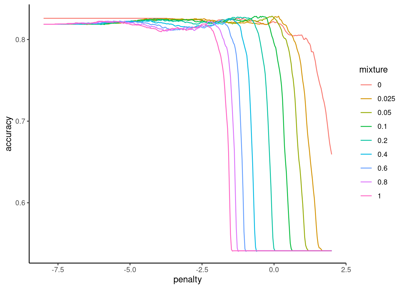

Question: Does the glmnet (regularized logistic regresssion) outperform a simple logistic regression? How would these two algorithms compare?

Show Answer

Remember that the linear model is a special case of glmnet where the penalty = 0.  
Here we are looking log penalty down to exp(-8) = 0.0003354626.  That is pretty 
close to 0 so an approximation of how the standard logistic regression would 
perform.  glmnet is slightly more accurate with its optimal hyperparameter values

Here we show the mean performance of the top 10 configurations

We use these performance estimates to select the top optimal values for the hyperparameters

We will choose the hyperparameter values from the configuration displayed in the first row of this table

collect_metrics(fits_full) |> 
  arrange(desc(mean)) |> 
  print(n = 10)

# A tibble: 2,700 × 8
   penalty mixture .metric  .estimator  mean     n std_err
     <dbl>   <dbl> <chr>    <chr>      <dbl> <int>   <dbl>
 1   0.929   0.05  accuracy binary     0.829   100 0.00610
 2   1.17    0.025 accuracy binary     0.829   100 0.00607
 3   0.509   0.1   accuracy binary     0.828   100 0.00618
 4   0.544   0.1   accuracy binary     0.828   100 0.00614
 5   0.622   0.1   accuracy binary     0.828   100 0.00618
 6   0.665   0.1   accuracy binary     0.828   100 0.00615
 7   0.526   0.1   accuracy binary     0.828   100 0.00611
 8   0.688   0.1   accuracy binary     0.828   100 0.00623
 9   0.869   0.05  accuracy binary     0.828   100 0.00623
10   1.03    0.025 accuracy binary     0.828   100 0.00601
   .config                
   <chr>                  
 1 Preprocessor1_Model0838
 2 Preprocessor1_Model0545
 3 Preprocessor1_Model1120
 4 Preprocessor1_Model1122
 5 Preprocessor1_Model1126
 6 Preprocessor1_Model1128
 7 Preprocessor1_Model1121
 8 Preprocessor1_Model1129
 9 Preprocessor1_Model0836
10 Preprocessor1_Model0541
# ℹ 2,690 more rows

Here we are storing that best configuration in an object so that we could later fit that configuration to the full dataset

(hp_best_full <- select_best(fits_full, n = 1))

# A tibble: 1 × 3
  penalty mixture .config                
    <dbl>   <dbl> <chr>                  
1   0.929    0.05 Preprocessor1_Model0838

Question: Tell me about bias if we use this mean performance from the 100 held-out folds as an estimate of how well that model fit to the full N will perform

Show Answer

There is some optimization bias in this performance estimate because we already
used these 100 held-out folds to select the best configuration.  This will be a 
second use of those folds.  This will lead us to over-estimate the models true 
performance in new data.  We would need a test set to remove this bias.

There is also some bias because we are using less that the full sample (k-1 folds) 
to estimate performance of a model that will eventually have N unique observations 
across all k folds.  This will lead  us to underestimate the true performance of 
our model in new data.

When we (eventually) compare the full and compact models, the presence of some bias may not be as important (and there will always be some bias anyway, because of the latter concern from the last slide).

We are focused on a relative comparison in performance across the two models so what is most important is that the bias is comparable for our assessments of the two models.

If we use validation data (e.g., our 100 held-out folds), there will be comparable optimization bias for both models so this may not be too problematic. We don’t need test data.

But before we go further, we need to have a compact model to compare to our full model

Here is a recipe to feature engineer features associated with this compact model

We can start with the full recipe and add one more step to remove (i.e., ablate) the features we want to evaluate
step_rm(contains("exer_")
All previous recipe steps remain the same

rec_compact <- rec_full |> 
  step_rm(contains("exer_"))

We need to select/tune hyperparameters for this new model

It has different complexity than the full model so it might need different (less?) regularization for optimal performance

fits_compact <- cache_rds(
  expr = {
    logistic_reg(penalty = tune(),
                 mixture = tune()) |> 
    set_engine("glmnet") |> 
    tune_grid(preprocessor = rec_compact,   # use recipe for compact model
              resamples = splits,
              grid = grid_glmnet,
              metrics = metric_set(accuracy))
  },
  rerun = rerun_setting,
  dir = "cache/011/",
  file = "fits_compact")

Confirm that we found a good set of hyperparameters

fits_compact |> 
  plot_hyperparameters(hp1 = "penalty", hp2 = "mixture", metric = "accuracy", 
                       log_hp1 = TRUE)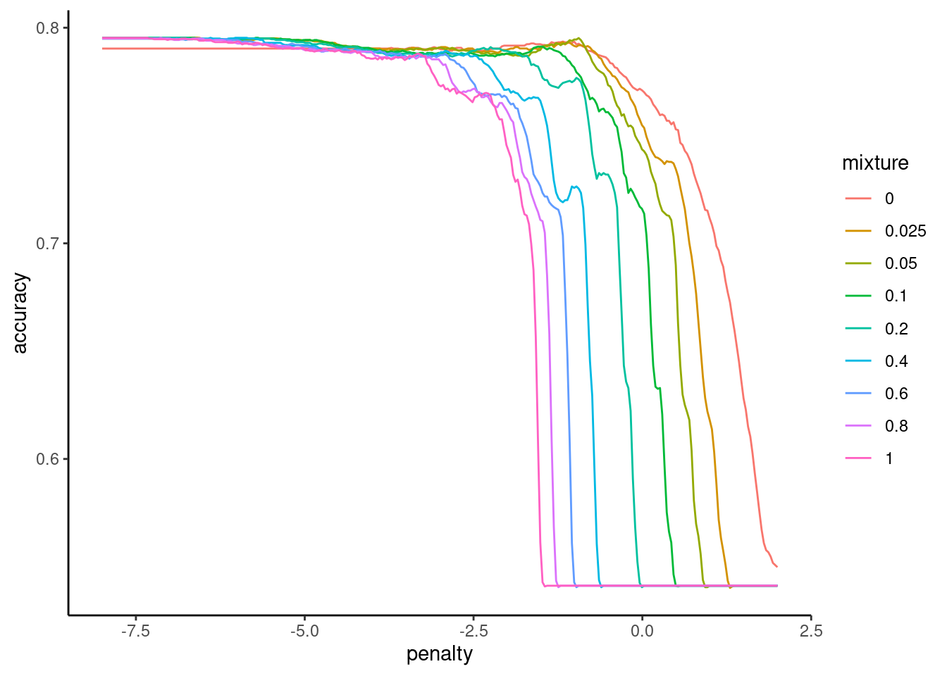

And here is our best configuration, for when we want to train the compact model on all the data at a later stage

(hp_best_compact <- select_best(fits_compact, n = 1))

# A tibble: 1 × 3
  penalty mixture .config                
    <dbl>   <dbl> <chr>                  
1 0.00116   0.025 Preprocessor1_Model0338

Now, here are accuracies for these two models assessed by 10 repeats of 10-fold

This is the mean performance for the best configuration
These means are based on 100 individual held-out folds

collect_metrics(fits_full) |> 
  arrange(desc(mean)) |> 
  slice(1)

# A tibble: 1 × 8
  penalty mixture .metric  .estimator  mean     n std_err
    <dbl>   <dbl> <chr>    <chr>      <dbl> <int>   <dbl>
1   0.929    0.05 accuracy binary     0.829   100 0.00610
  .config                
  <chr>                  
1 Preprocessor1_Model0838

collect_metrics(fits_compact) |> 
  arrange(desc(mean)) |> 
  slice(1)

# A tibble: 1 × 8
  penalty mixture .metric  .estimator  mean     n std_err
    <dbl>   <dbl> <chr>    <chr>      <dbl> <int>   <dbl>
1 0.00116   0.025 accuracy binary     0.795   100 0.00706
  .config                
  <chr>                  
1 Preprocessor1_Model0338

The compact model is less accurate but…..

A simple descriptive comparison is not sufficient to justify the use of a costly test
We need to be more confident that the test really improves screening in all possible held out samples from our dataset
And by how much?
How can we compare these two models?

11.6 Nadeau and Bengio (2003) Correlated t-test

We have 100 held-out accuracies for each model.

Could we compare these?

Well, we have the same 100 held-out samples (we used the same splits) for both compact and full models so these two sets of accuracies (for each of the two models) should be considered paired/repeated.

Not a problem, we could use paired samples t-test
Easiest to think about this paired test as testing if the differences in accuracy for each of the 100 held out sets == 0. That removes the lack of independence from using the sample 100 held-out sets twice

BUT these 100 differences are still not independent

Each have been estimated using models that were fit with overlapping observations (the held in sets were fit with many of the same observations for each of the k-1 held in folds)
If we ignore this violation and simply do a paired-samples t-test, we will have inflation of alpha

Nadeau and Bengio (2003) (see pdf) and Bouckaert (2003) (see pdf) have explored the degree of dependence among performance estimates using resampling.

This was originally done for repeated random train/test splits (e.g., 90/10 splits) but is now also used when doing repeated k-fold.

The classic paired t-test has the following formula

\(t = \frac{\overline{x} - 0}{\sqrt{\hat{\sigma^2}*\frac{1}{n}}}\)

The standard error for the difference (denominator of the t-statistic formula) is too small

Nadeau and Benigo adjusted it by \(\frac{\rho}{1-\rho}\) where \(\rho = \frac{n_{test}}{n_{total}}\) or equivalent \(\frac{1}{k}\)

This adjustment yields:

\(t = \frac{\overline{x} - 0}{\sqrt{\hat{\sigma^2}*(\frac{1}{n} + \frac{\rho}{1-\rho})}}\)

Let’s perform this correlated t-test to compare our compact and full models

We first need to extract the 100 held-out folds from fits_full and fits_compact

When we have used collect_metrics() in the past, we always used the default for summarize (which is TRUE). This gave us average performance for each model configuration across all the held-out folds. But the individual folds for each configuration are in that object too

Our best model configuration for the full model was

hp_best_full

# A tibble: 1 × 3
  penalty mixture .config                
    <dbl>   <dbl> <chr>                  
1   0.929    0.05 Preprocessor1_Model0838

hp_best_full$.config

[1] "Preprocessor1_Model0838"

We can see that label assigned to that specific configuration in the .config column. We can use that to pull out the 100 folds for that configuration

cv_full <- collect_metrics(fits_full, summarize = FALSE) |> 
  filter(.config == hp_best_full$.config) |> 
  pull(.estimate)

cv_full |> print()

  [1] 0.8387097 0.9032258 0.8387097 0.8709677 0.8000000 0.7333333 0.8666667
  [8] 0.7333333 0.8666667 0.8275862 0.8064516 0.8064516 0.7741935 0.8709677
 [15] 0.8666667 0.8666667 0.8000000 0.8000000 0.7666667 0.8965517 0.8064516
 [22] 0.8387097 0.8709677 0.8709677 0.9000000 0.9000000 0.9000000 0.6666667
 [29] 0.7666667 0.7586207 0.9354839 0.8064516 0.8709677 0.7419355 0.7666667
 [36] 0.9333333 0.7666667 0.7666667 0.9000000 0.7586207 0.7419355 0.8387097
 [43] 0.8709677 0.9354839 0.8333333 0.9000000 0.8333333 0.7333333 0.7666667
 [50] 0.8275862 0.8387097 0.9354839 0.8064516 0.7741935 0.8333333 0.8000000
 [57] 0.9000000 0.7666667 0.9000000 0.7931034 0.7741935 0.8387097 0.8387097
 [64] 0.9032258 0.9000000 0.8000000 0.8666667 0.7000000 0.8333333 0.8620690
 [71] 0.7741935 0.8387097 0.8387097 0.8064516 0.7000000 0.9000000 0.8333333
 [78] 0.8666667 0.8666667 0.8275862 0.8387097 0.8387097 0.8709677 0.8387097
 [85] 0.7333333 0.8000000 0.8000000 0.9333333 0.7666667 0.8620690 0.6774194
 [92] 0.7741935 0.9032258 0.8709677 0.8666667 0.9333333 0.8333333 0.8666667
 [99] 0.7666667 0.8275862

And lets get the 100 folds for the compact model

hp_best_compact

# A tibble: 1 × 3
  penalty mixture .config                
    <dbl>   <dbl> <chr>                  
1 0.00116   0.025 Preprocessor1_Model0338

hp_best_compact$.config

[1] "Preprocessor1_Model0338"

cv_compact <- collect_metrics(fits_compact, summarize = FALSE) |> 
  filter(.config == hp_best_compact$.config) |> 
  pull(.estimate)

cv_full |> print()

  [1] 0.8387097 0.9032258 0.8387097 0.8709677 0.8000000 0.7333333 0.8666667
  [8] 0.7333333 0.8666667 0.8275862 0.8064516 0.8064516 0.7741935 0.8709677
 [15] 0.8666667 0.8666667 0.8000000 0.8000000 0.7666667 0.8965517 0.8064516
 [22] 0.8387097 0.8709677 0.8709677 0.9000000 0.9000000 0.9000000 0.6666667
 [29] 0.7666667 0.7586207 0.9354839 0.8064516 0.8709677 0.7419355 0.7666667
 [36] 0.9333333 0.7666667 0.7666667 0.9000000 0.7586207 0.7419355 0.8387097
 [43] 0.8709677 0.9354839 0.8333333 0.9000000 0.8333333 0.7333333 0.7666667
 [50] 0.8275862 0.8387097 0.9354839 0.8064516 0.7741935 0.8333333 0.8000000
 [57] 0.9000000 0.7666667 0.9000000 0.7931034 0.7741935 0.8387097 0.8387097
 [64] 0.9032258 0.9000000 0.8000000 0.8666667 0.7000000 0.8333333 0.8620690
 [71] 0.7741935 0.8387097 0.8387097 0.8064516 0.7000000 0.9000000 0.8333333
 [78] 0.8666667 0.8666667 0.8275862 0.8387097 0.8387097 0.8709677 0.8387097
 [85] 0.7333333 0.8000000 0.8000000 0.9333333 0.7666667 0.8620690 0.6774194
 [92] 0.7741935 0.9032258 0.8709677 0.8666667 0.9333333 0.8333333 0.8666667
 [99] 0.7666667 0.8275862

NOTE: It is important that these are the SAME splits for both model configurations

Now we can compare these 100 folds across the two models using the correlated t-test

Define a function for Nadeau and Bengio (2003) correlated t-test

# included in fun_ml.R
nb_correlated_t_test <- function(cv_full, cv_compact, k = 10){

    diffs <- cv_full - cv_compact
    n <- length(diffs)
    mean_diff <- mean(diffs)
    var_diffs <- var(diffs)
    proportion_test <- 1 / k
    proportion_train <- 1 - proportion_test
    correction <- (1 / n) + (proportion_test / proportion_train)
    se = sqrt(correction * var_diffs)

    t = abs(mean_diff/se)
    p_value <- 2 * pt(t, n - 1, lower.tail = FALSE)
    tibble(mean_diff = mean_diff, se = se, t = t, df = n - 1, p_value = p_value)
}

Calculate the t-test.

In this instance we likely want a one-tailed test (though of course, that should have been planned in advanced and ideally pre-registered!).

My function returns a two-tailed p-value so we should cut it in half.

nb_correlated_t_test(cv_full, 
                     cv_compact, 
                     k = 10)

# A tibble: 1 × 5
  mean_diff     se     t    df p_value
      <dbl>  <dbl> <dbl> <dbl>   <dbl>
1    0.0333 0.0271  1.23    99   0.222

The improvement in prediction accuracy associated with the use of our exercise test protocol is not significant (p = 0.11, one-tailed).

11.7 Bayesian estimation for model comparisons

Benavoli et al. (2017) critique the many shortcomings wrt the frequentist approach, and I must admit, I am mostly convinced

NHST does not provide the probabilities of the null and alternative hypotheses.
- That is what we want
- NHST gives us the probability of our data given the null
NHST focuses on a point-wise comparison (no difference) that is almost never true.
NHST yields no information about the null hypothesis (i.e., when we fail to reject)
The inference depends on the sampling and testing intention (think about Bonferonni correction)

They suggest to use Bayesian parameter estimation as alternative to the t-test. Bayesian estimation has now been included in tidymodels in the tidyposterior package using the perf_mod() function.

You can (and should!) read more about this implementation of Bayesian Estimation in the associated vignette AND by reading the help materials on perf_mod()

Using this approach, we will estimate the posterior probability for values associated with specific parameters of interest. For our goals, we will care about estimates of three parameters

The accuracy of the full model
The accuracy of the compact model
The difference in accuracies between these two models.

We want to determine the posterior probabilities associated with ranges of values for each of these three model performance parameters estimates. We can then use these posterior probability distributions to determine that probability that the accuracy of the full model is greater than the accuracy of the compact model.

In addition, we can also determine if the increased accuracy of the full model is meaningful (i.e., practically important).

To accomplish this latter goal, we will:

Specify a Region of Practical Equivalence (a better alternative to the point-wise null in NHST)
- I will define classifiers whose performance are within +-1% as equivalent (not meaningfully different from each other) for our example
- Not worth the effort if my test doesn’t improve screening accuracy by at least this

To estimate posterior probabilities for these three parameter estimates, we need to

set prior probabilities for these parameter estimates. These should be broad/uninformative in most instances unless you have substantial prior information about credible values.
Collect data on these estimates. This will be the same as before - the 100 estimates of accuracy using 10x10 fold CV for both the full and compact models.

Using these priors and these data, we can derive the posterior probabilities for our three performance estimates

Lets do this step by step. We will use the tidyposterior package. It in not included when we load tidymodels so we will load it now

library(tidyposterior)

We need to make a dataframe of our 100 performance estimates for the full and compact models. Here is the code to do this using our previous resamples of our models

Make dataframes of the accuracies from the full model and the compact model

accuracy_full <- collect_metrics(fits_full, summarize = FALSE) |> 
  filter(.config == hp_best_full$.config) |>   # as before - the best config
  select(id, id2, full = .estimate) |> 
  print()

# A tibble: 100 × 3
   id       id2     full
   <chr>    <chr>  <dbl>
 1 Repeat01 Fold01 0.839
 2 Repeat01 Fold02 0.903
 3 Repeat01 Fold03 0.839
 4 Repeat01 Fold04 0.871
 5 Repeat01 Fold05 0.8  
 6 Repeat01 Fold06 0.733
 7 Repeat01 Fold07 0.867
 8 Repeat01 Fold08 0.733
 9 Repeat01 Fold09 0.867
10 Repeat01 Fold10 0.828
# ℹ 90 more rows

accuracy_compact <- collect_metrics(fits_compact, summarize = FALSE) |> 
  filter(.config == hp_best_compact$.config) |>   # as before - the best config
  select(id, id2, compact = .estimate) |> 
  print()

# A tibble: 100 × 3
   id       id2    compact
   <chr>    <chr>    <dbl>
 1 Repeat01 Fold01   0.774
 2 Repeat01 Fold02   0.806
 3 Repeat01 Fold03   0.774
 4 Repeat01 Fold04   0.806
 5 Repeat01 Fold05   0.867
 6 Repeat01 Fold06   0.7  
 7 Repeat01 Fold07   0.733
 8 Repeat01 Fold08   0.9  
 9 Repeat01 Fold09   0.7  
10 Repeat01 Fold10   0.759
# ℹ 90 more rows

Now we need to join these dataframes, matching on repeat and fold ids

resamples <- accuracy_full |> 
  full_join(accuracy_compact, by = c("id", "id2")) |> 
  print()

# A tibble: 100 × 4
   id       id2     full compact
   <chr>    <chr>  <dbl>   <dbl>
 1 Repeat01 Fold01 0.839   0.774
 2 Repeat01 Fold02 0.903   0.806
 3 Repeat01 Fold03 0.839   0.774
 4 Repeat01 Fold04 0.871   0.806
 5 Repeat01 Fold05 0.8     0.867
 6 Repeat01 Fold06 0.733   0.7  
 7 Repeat01 Fold07 0.867   0.733
 8 Repeat01 Fold08 0.733   0.9  
 9 Repeat01 Fold09 0.867   0.7  
10 Repeat01 Fold10 0.828   0.759
# ℹ 90 more rows

Now we can use perf_mod() to derive the posterior probabilites for the accuracy of each of these two models

We need to specify a model with parameters in formula. Here we indicate that we have a multi-level model with repeated observation of accuracy across folds (id2) nested within repeats (id). This handles dependence associated with repeated observations of accuracy using similar models in k-fold cv.
We are interested in the intercept from this model listed in formula. The intercept value will represent the accuracy estimate for each model.
The default for perf_mod() will be to constrain the variances of the intercept parameter estimate to be the same across models. This may be fine for some performance metrics (e.g., rmse) but for binary accuracy the variance is dependent on the mean. Therefore we allow these variances to be different using hetero_var = TRUE
In some instances (e..g., rmse), we may want to allow the errors in our model to be something other than Gaussian (though this is often a reasonable assumption by the central limit theorem). You can change the family for the errors if needed. See vignette and help on perf_mod(). Here, we use the default Gaussian distribution.
This is an iterative process using a Markov chain Monte Carlo method (Hamilton Monte Carlo) so we need to set a seed (for reproducibility), and the number of iterations and chains (beyond the scope of this course to dive into this method). I provide default values for iter and chains because you may need to increase these in some instances for the method to converge on valid values. You can often address converge and other warnings by increasing iter, chains or adapt_delta. You can read more about these warnings and issues here, here, here, and here to start.

Here is the code

set.seed(101)
pp <- cache_rds(
  expr = {
    perf_mod(resamples, 
            formula = statistic ~ model + (1 | id2/id),
            # defaults but may require increases
            iter = 2000, chains = 4,  
            # for more Gaussian distribution of accuracy
            transform = tidyposterior::logit_trans,
            hetero_var = TRUE, # for accuracy
            family = gaussian, # default but could change depending on DV
            # increase adapt_delta (e.g., .99, .999) to 
            # fix divergent transitions
            adapt_delta = .99)  
  },
rerun = rerun_setting,
dir = "cache/011/",
file = "pp")


SAMPLING FOR MODEL 'continuous' NOW (CHAIN 1).
Chain 1: 
Chain 1: Gradient evaluation took 0.000766 seconds
Chain 1: 1000 transitions using 10 leapfrog steps per transition would take 7.66 seconds.
Chain 1: Adjust your expectations accordingly!
Chain 1: 
Chain 1: 
Chain 1: Iteration:    1 / 2000 [  0%]  (Warmup)
Chain 1: Iteration:  200 / 2000 [ 10%]  (Warmup)
Chain 1: Iteration:  400 / 2000 [ 20%]  (Warmup)
Chain 1: Iteration:  600 / 2000 [ 30%]  (Warmup)
Chain 1: Iteration:  800 / 2000 [ 40%]  (Warmup)
Chain 1: Iteration: 1000 / 2000 [ 50%]  (Warmup)
Chain 1: Iteration: 1001 / 2000 [ 50%]  (Sampling)
Chain 1: Iteration: 1200 / 2000 [ 60%]  (Sampling)
Chain 1: Iteration: 1400 / 2000 [ 70%]  (Sampling)
Chain 1: Iteration: 1600 / 2000 [ 80%]  (Sampling)
Chain 1: Iteration: 1800 / 2000 [ 90%]  (Sampling)
Chain 1: Iteration: 2000 / 2000 [100%]  (Sampling)
Chain 1: 
Chain 1:  Elapsed Time: 3.385 seconds (Warm-up)
Chain 1:                2.268 seconds (Sampling)
Chain 1:                5.653 seconds (Total)
Chain 1: 

SAMPLING FOR MODEL 'continuous' NOW (CHAIN 2).
Chain 2: 
Chain 2: Gradient evaluation took 4.6e-05 seconds
Chain 2: 1000 transitions using 10 leapfrog steps per transition would take 0.46 seconds.
Chain 2: Adjust your expectations accordingly!
Chain 2: 
Chain 2: 
Chain 2: Iteration:    1 / 2000 [  0%]  (Warmup)
Chain 2: Iteration:  200 / 2000 [ 10%]  (Warmup)
Chain 2: Iteration:  400 / 2000 [ 20%]  (Warmup)
Chain 2: Iteration:  600 / 2000 [ 30%]  (Warmup)
Chain 2: Iteration:  800 / 2000 [ 40%]  (Warmup)
Chain 2: Iteration: 1000 / 2000 [ 50%]  (Warmup)
Chain 2: Iteration: 1001 / 2000 [ 50%]  (Sampling)
Chain 2: Iteration: 1200 / 2000 [ 60%]  (Sampling)
Chain 2: Iteration: 1400 / 2000 [ 70%]  (Sampling)
Chain 2: Iteration: 1600 / 2000 [ 80%]  (Sampling)
Chain 2: Iteration: 1800 / 2000 [ 90%]  (Sampling)
Chain 2: Iteration: 2000 / 2000 [100%]  (Sampling)
Chain 2: 
Chain 2:  Elapsed Time: 4.391 seconds (Warm-up)
Chain 2:                2.2 seconds (Sampling)
Chain 2:                6.591 seconds (Total)
Chain 2: 

SAMPLING FOR MODEL 'continuous' NOW (CHAIN 3).
Chain 3: 
Chain 3: Gradient evaluation took 4.3e-05 seconds
Chain 3: 1000 transitions using 10 leapfrog steps per transition would take 0.43 seconds.
Chain 3: Adjust your expectations accordingly!
Chain 3: 
Chain 3: 
Chain 3: Iteration:    1 / 2000 [  0%]  (Warmup)
Chain 3: Iteration:  200 / 2000 [ 10%]  (Warmup)
Chain 3: Iteration:  400 / 2000 [ 20%]  (Warmup)
Chain 3: Iteration:  600 / 2000 [ 30%]  (Warmup)
Chain 3: Iteration:  800 / 2000 [ 40%]  (Warmup)
Chain 3: Iteration: 1000 / 2000 [ 50%]  (Warmup)
Chain 3: Iteration: 1001 / 2000 [ 50%]  (Sampling)
Chain 3: Iteration: 1200 / 2000 [ 60%]  (Sampling)
Chain 3: Iteration: 1400 / 2000 [ 70%]  (Sampling)
Chain 3: Iteration: 1600 / 2000 [ 80%]  (Sampling)
Chain 3: Iteration: 1800 / 2000 [ 90%]  (Sampling)
Chain 3: Iteration: 2000 / 2000 [100%]  (Sampling)
Chain 3: 
Chain 3:  Elapsed Time: 3.781 seconds (Warm-up)
Chain 3:                2.245 seconds (Sampling)
Chain 3:                6.026 seconds (Total)
Chain 3: 

SAMPLING FOR MODEL 'continuous' NOW (CHAIN 4).
Chain 4: 
Chain 4: Gradient evaluation took 3.8e-05 seconds
Chain 4: 1000 transitions using 10 leapfrog steps per transition would take 0.38 seconds.
Chain 4: Adjust your expectations accordingly!
Chain 4: 
Chain 4: 
Chain 4: Iteration:    1 / 2000 [  0%]  (Warmup)
Chain 4: Iteration:  200 / 2000 [ 10%]  (Warmup)
Chain 4: Iteration:  400 / 2000 [ 20%]  (Warmup)
Chain 4: Iteration:  600 / 2000 [ 30%]  (Warmup)
Chain 4: Iteration:  800 / 2000 [ 40%]  (Warmup)
Chain 4: Iteration: 1000 / 2000 [ 50%]  (Warmup)
Chain 4: Iteration: 1001 / 2000 [ 50%]  (Sampling)
Chain 4: Iteration: 1200 / 2000 [ 60%]  (Sampling)
Chain 4: Iteration: 1400 / 2000 [ 70%]  (Sampling)
Chain 4: Iteration: 1600 / 2000 [ 80%]  (Sampling)
Chain 4: Iteration: 1800 / 2000 [ 90%]  (Sampling)
Chain 4: Iteration: 2000 / 2000 [100%]  (Sampling)
Chain 4: 
Chain 4:  Elapsed Time: 3.611 seconds (Warm-up)
Chain 4:                3.844 seconds (Sampling)
Chain 4:                7.455 seconds (Total)
Chain 4:

Warning: Bulk Effective Samples Size (ESS) is too low, indicating posterior means and medians may be unreliable.
Running the chains for more iterations may help. See
https://mc-stan.org/misc/warnings.html#bulk-ess

Warning: Tail Effective Samples Size (ESS) is too low, indicating posterior variances and tail quantiles may be unreliable.
Running the chains for more iterations may help. See
https://mc-stan.org/misc/warnings.html#tail-ess

In contrast to the NHST approach, we now have what we really want - posterior probabilities. Lets look at them

We can view the posterior probability distributions using an autoplot method for perf_mod objects.

These density plots tell how probable various values are for the accuracy of each model
The probabilities associated with any region of the curve is equal to the area under that curve for that region. This will tell you the probability associated with that range of values for accuracy.
You can easily see in this instance that the probable values for accuracy are higher generally for full model than the compact model

pp |> autoplot()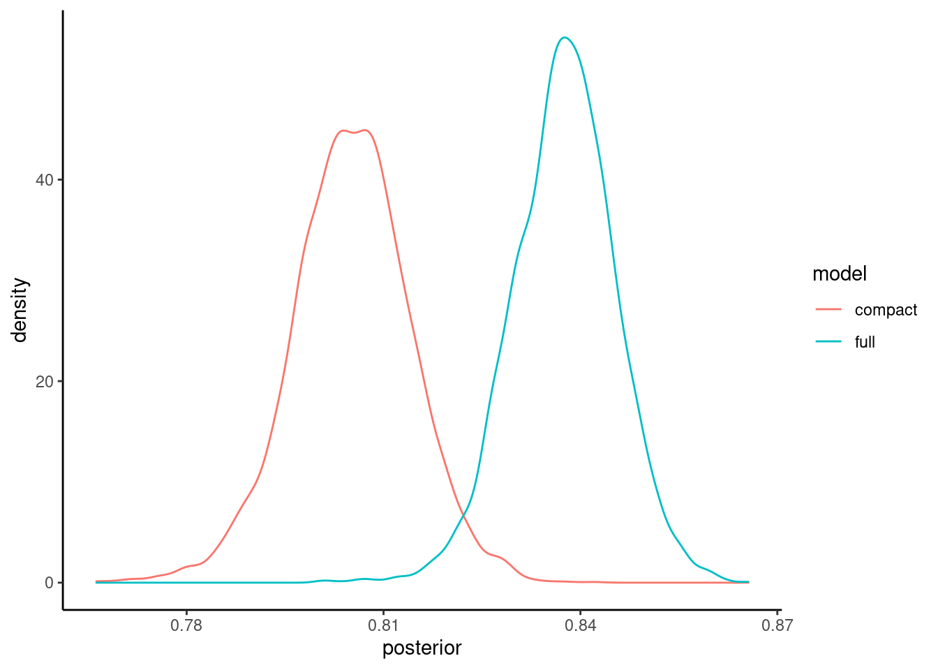

You will likely want to publish a figure showing these posterior probability distributions so you may want to fine tune the plots. Here are some code options using ggplot

Here is the same density plots using ggplot so you can now edit to adjust as you like

pp |> 
  tidy(seed = 123) |> 
  mutate(model = fct_inorder(model)) |>
  ggplot() + 
  geom_density(aes(x = posterior, color = model) )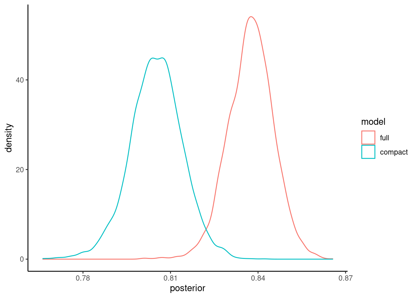

We are actually sampling from the posterior distribution so it might make more sense to display these as histograms rather than density plots

pp |> 
  tidy(seed = 123) |> 
  mutate(model = fct_inorder(model)) |>
  ggplot() + 
  geom_histogram(aes(x = posterior, fill = model), color = "white", alpha = 0.4,
                 bins = 50, position = "identity")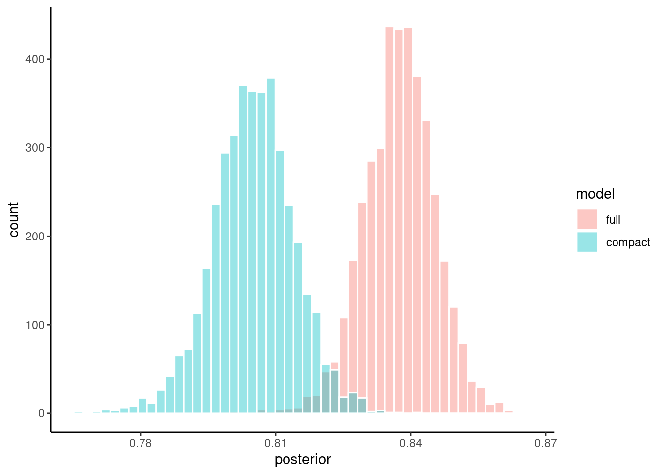

Or maybe you want to facet the histograms if the overlap is difficulty to view

pp |> 
  tidy(seed = 123) |> 
  mutate(model = fct_inorder(model)) |>
  ggplot(aes(x = posterior)) + 
  geom_histogram(color = "white", fill = "blue", bins = 30) + 
  facet_wrap(~ model, ncol = 1)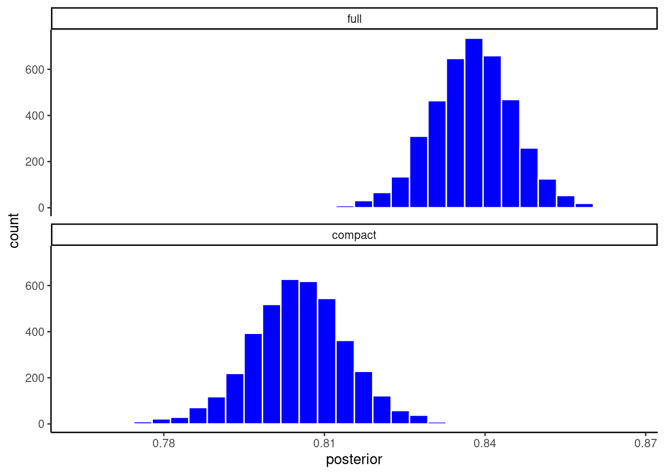

We can also calculate the 95% Higher Density Intervals (aka, 95% Credible Intervals; the Bayesian alternative to the 95% Confidence Intervals) for the accuracy of each model. This is the range of parameter estimate values that include 95% of the credible values. Kruschke described this in the assigned reading.

pp |> tidy(seed = 123) |> summary()

# A tibble: 2 × 4
  model    mean lower upper
  <chr>   <dbl> <dbl> <dbl>
1 compact 0.805 0.790 0.820
2 full    0.838 0.825 0.850

But what we really want is derive the posterior probability for the difference in accuracy between the two models. This will let us determine credible values for the magnitude of the difference and determine if this difference is meaningful.

We said early that we would define a ROPE of +-.01 around zero. The models are only meaningful different if their accuracies differ by at least 1%

Lets visualize the posterior probability distribution for the difference along with this ROPE using the built in autoplot function

pp |> contrast_models(seed = 4) |> autoplot(size = .01)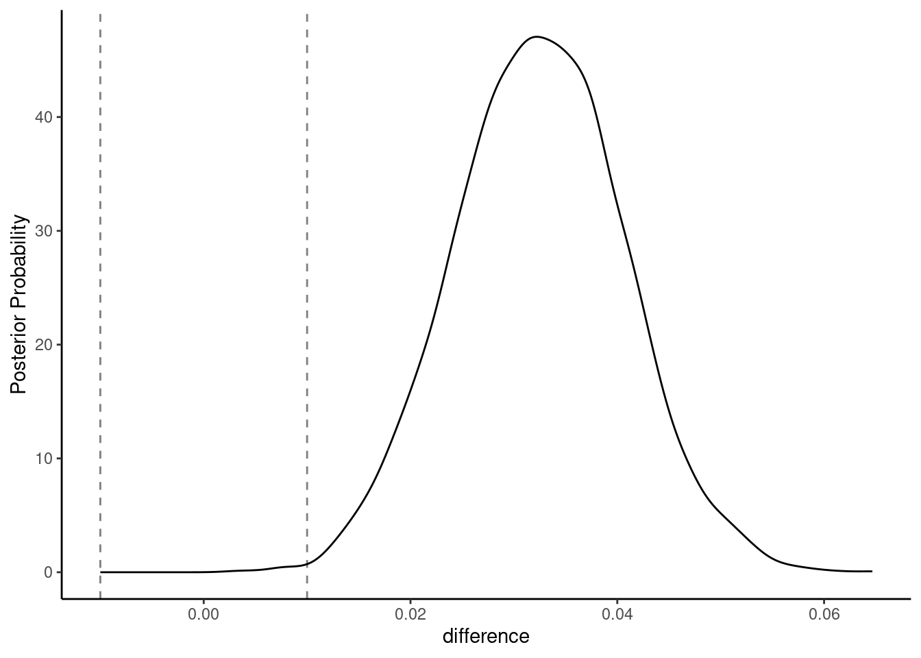

We could make more pretty plots directly in ggplot

pp |> 
  contrast_models(seed = 4) |> 
  ggplot() +
  geom_density(aes(x = difference), color = "blue")+
  geom_vline(aes(xintercept = -.01), linetype = "dashed") + 
  geom_vline(aes(xintercept = .01), linetype = "dashed")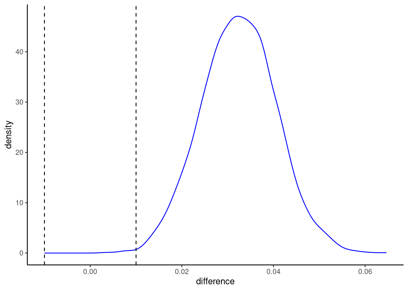

or my preferred histogram

pp |> 
  contrast_models(seed = 4) |> 
  ggplot(aes(x = difference)) + 
  geom_histogram(bins = 50, color = "white", fill = "blue")+
  geom_vline(aes(xintercept = -.01), linetype = "dashed") + 
  geom_vline(aes(xintercept = .01), linetype = "dashed")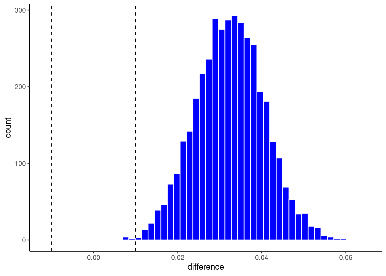

But perhaps most important, lets calculate the probability that the full model is more accurate than the compact model

The mean increase in accuracy is in the meancolumn
The 95% HDI is given by lower and upper
The probability that the full model is meaningfully higher than the compact model (i.e., what proportion of the credible values are above the ROPE) is in the prac_pos column.

pp |> contrast_models(seed = 4) |> summary(size = .01)

# A tibble: 1 × 9
  contrast        probability   mean  lower  upper  size pract_neg pract_equiv
  <chr>                 <dbl>  <dbl>  <dbl>  <dbl> <dbl>     <dbl>       <dbl>
1 full vs compact           1 0.0324 0.0189 0.0458  0.01         0     0.00225
  pract_pos
      <dbl>
1     0.998

Alternatively, using the approach proposed by Kruschke (2018), you can conclude that the full model is meaningfully better than the compact model if the 95% HDI is fully above the ROPE. This is also true!

Finally, in some instances, you may not want to use the ROPE.

Instead, you may simply want the posterior probability that the full model performs better than the compact model.
This is probability is provided in the probability column of the table.
You can also set the size of the ROPE to 0 (though not necessary)

pp |> contrast_models(seed = 4) |> summary(size = 0)

# A tibble: 1 × 9
  contrast        probability   mean  lower  upper  size pract_neg pract_equiv
  <chr>                 <dbl>  <dbl>  <dbl>  <dbl> <dbl>     <dbl>       <dbl>
1 full vs compact           1 0.0324 0.0189 0.0458     0        NA          NA
  pract_pos
      <dbl>
1        NA

11.8 Feature Importance

There as been increasing focus on improving the interpretability of machine learning models that we are using.

There are numerous reasons to want to better understand why our models make the predictions that they do.

The growing set of tools to interpret our models can help address our explanatory questions
But they can also help us find errors in our models
And they can detect possible bias (we will focus explicitly on algorithmic bias in later units)

Feature importance metrics are an important tool to better understand how our models work.

These metrics help us understand which features in our models contribute most to the predictions that the model makes.

For some models, interpretation and identification of important features is easy.

For example, if we standardize the features in a glm or glmnet model, we can interpret the absolute magnitude of the parameter estimates (i.e., the coefficients) as an index of the global (i.e., across all observations) importance of each feature.

You can use the vip package to extract these model-specific feature importance metrics, but you can often just get them directly from the model as well
More info on the use of vip package is available elsewhere

But for other models, we need different approaches.

There are many model-agnostic (i.e., can be used across all statistical algorithms) approaches to quantify the importance of a feature, but we will focus on two:

Permutation Feature Importance
Shapley Values

We follow recommendations from the tidymodels folks and use the DALEX and DALEXtra packages for model agnostic approaches to feature importance.

library(DALEX, exclude= "explain")

Welcome to DALEX (version: 2.4.3).
Find examples and detailed introduction at: http://ema.drwhy.ai/

library(DALEXtra)

Lets first get some coding issues accomplished before we dig into the details of the two feature importance metrics

To calculate these importance metrics, we will need access to the raw features and outcome.

rec_full_prep <- rec_full |> 
  prep(data_all)

feat_full <-  rec_full_prep |> 
  bake(data_all)

And we now will need to fit the full model trained on all the data

fit_full <- 
  logistic_reg(penalty = hp_best_full$penalty,
               mixture = hp_best_full$mixture) |> 
  set_engine("glmnet") |> 
  fit(disease ~ ., data = feat_full)

We will need to have a df for the features (without the outcome) and a separate vector for the outcome

features are easy. Just select out the outcome

x <- feat_full |> select(-disease)

For outcome, we need to convert to 0/1 (if classification), and then pull the vector out of the dataframe

y <- feat_full |> 
  mutate(disease = if_else(disease == "yes", 1, 0)) |> 
  pull(disease)

We also need a specific predictor function that will work with the DALEX package

We will write a custom function that “wraps” around our tidymodels predict() function

DALEX needs:

the prediction function to have two parameters named model and newdata
the prediction function must return a vector of probabilites for the positive class for classification problems (for regression, it simply returns a vector of the predicted values for \(y\))

predict_wrapper <- function(model, newdata) {
  predict(model, newdata, type = "prob") |> 
    pull(.pred_yes)
}

We will also need an explainer object based on our model and data

The explain_tidymodels() function in DALEXtra will create (and check) this object for us.

explain_full <- explain_tidymodels(fit_full, # our model object 
                                   data = x, # df with features without outcome
                                   y = y, # outcome vector
                                   # our custom predictor function
                                   predict_function = predict_wrapper)

Preparation of a new explainer is initiated
  -> model label       :  model_fit  (  default  )
  -> data              :  303  rows  17  cols 
  -> data              :  tibble converted into a data.frame 
  -> target variable   :  303  values 
  -> predict function  :  predict_function 
  -> predicted values  :  No value for predict function target column. (  default  )
  -> model_info        :  package parsnip , ver. 1.1.0.9004 , task classification (  default  ) 
  -> predicted values  :  numerical, min =  0.2574049 , mean =  0.458745 , max =  0.7385297  
  -> residual function :  residual_function 
  -> residuals         :  numerical, min =  0 , mean =  0 , max =  0  
  A new explainer has been created!

Finally, we need to define a custom function for our performance metric as well

It needs to have two parameters: observed and predicted
We can create a wrapper function around accuracy_vec() to fit these needs
For accuracy, we need to transform the predicted probabilites from our prediction function to class predictions (e.g.. yes/no)
And because we converted our labels to 0/1 in the outcome vector, we need to transform observed back to yes/no as well

accuracy_wrapper <- function(observed, predicted) {
  observed <- fct(if_else(observed == 1, "yes", "no"),
                  levels = c("yes", "no"))
  predicted <- fct(if_else(predicted > .5, "yes", "no"), levels  = c("yes", "no"))
  accuracy_vec(observed, predicted)
}

We are now ready to calculate feature importance metrics

11.8.1 Permutation Feature Importance

The first model agnostic approach to calculating feature important is called Permutation Feature Importance

This approach is very straight forward. This approach says - if we want to calculate the importance of any specific feature, we can compare our performance metric using the original features to the performance metric we get if we permute (i.e., shuffle) the values for the feature we are evaluating.

By randomly shuffling the values for the feature, we break the relationship between that feature and the outcome so it no longer contributes to the predictions. If performance doesn’t change much, then that feature is not important. If performance goes down a lot, the feature is important.

The function can provide raw performance (will give us performance for the non-permuted model and then performance for the model with each feature permuted, one at a time)
difference performance measure, which is the difference between the permuted model and the non-permuted mode, separately for each feature
ratio performance measure, which is (\(\frac{permuted}{original}\)), separately for each feature

To calculate accuracy after permuting each feature, we use model_parts(). We pass in

our explainer object
set the type (raw in this example)
indicate our custom accuracy function
set B to indicate number of permutations to perform

set.seed(123456)
imp_permute <- model_parts(explain_full, 
                               type = "raw", 
                               loss_function = accuracy_wrapper,
                               B = 100)

Lets look at what this function returns

the first row contains the accuracy for the full model (with no features permuted)
last row is a baseline models (performance with all features permuted)
Other row show the accuracy of the model when that specific feature is permuted

imp_permute

                       variable mean_dropout_loss     label
1                  _full_model_         0.8382838 model_fit
2                            ca         0.7944224 model_fit
3         thal_reversabledefect         0.8002640 model_fit
4                  exer_ang_yes         0.8116172 model_fit
5                   exer_max_hr         0.8161386 model_fit
6               exer_st_depress         0.8189769 model_fit
7            exer_st_slope_flat         0.8237294 model_fit
8                cp_non_anginal         0.8249505 model_fit
9                      sex_male         0.8304620 model_fit
10                  cp_atyp_ang         0.8338284 model_fit
11                      rest_bp         0.8351155 model_fit
12                          age         0.8355116 model_fit
13 rest_ecg_ventric_hypertrophy         0.8378878 model_fit
14                         chol         0.8382838 model_fit
15                 fbs_elevated         0.8382838 model_fit
16            rest_ecg_wave_abn         0.8382838 model_fit
17      exer_st_slope_downslope         0.8382838 model_fit
18             thal_fixeddefect         0.8382838 model_fit
19                   _baseline_         0.5082508 model_fit

We can use the built in plot function from DALEX to display this

plot(imp_permute)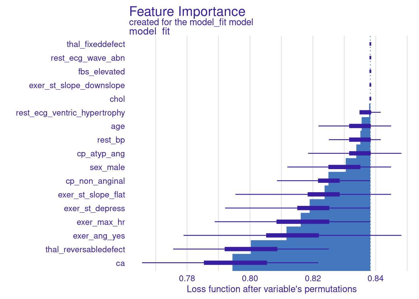

Or we can plot it directly. Here is an example from the tidymodels folks

full_model <- imp_permute |>  
    filter(variable == "_full_model_")
  
imp_permute |> 
  filter(variable != "_full_model_",
         variable != "_baseline_") |> 
  mutate(variable = fct_reorder(variable, dropout_loss)) |> 
  ggplot(aes(dropout_loss, variable)) +
  geom_vline(data = full_model, aes(xintercept = dropout_loss),
             linewidth = 1.4, lty = 2, alpha = 0.7) +
  geom_boxplot(fill = "#91CBD765", alpha = 0.4) +
  theme(legend.position = "none") +
  labs(x = "accuracy", 
       y = NULL,  fill = NULL,  color = NULL)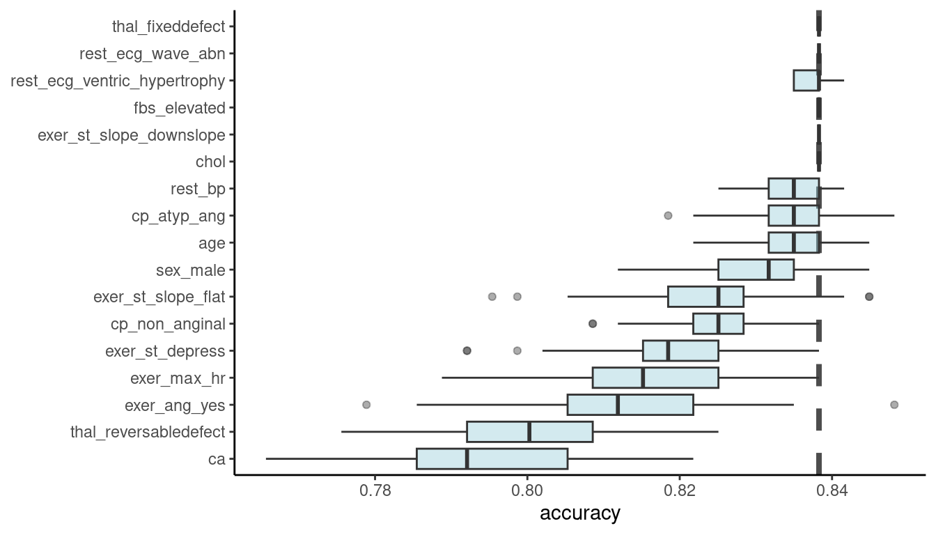

We can also permute a set of features to quantify the contribution of the full set

This is what we would want for our example, were we want to know the contribution of the four features that represent our exercise test.

To do this, we pass in a list of vectors of the groups. Here we provide just one group that we name exer_test

set.seed(123456)
imp_permute_group <- model_parts(explain_full, 
                               type = "raw", 
                               loss_function = accuracy_wrapper,
                               B = 100,
                               variable_groups = list(exer_test = 
                                                        c("exer_ang_yes",
                                                          "exer_max_hr",
                                                          "exer_st_depress", 
                                                          "exer_st_slope_downslope")))

The results show that permuting these four features as a set drops accuracy from 0.838 to 0.738

imp_permute_group

      variable mean_dropout_loss     label
1 _full_model_         0.8382838 model_fit
2    exer_test         0.7128713 model_fit
3   _baseline_         0.5145215 model_fit

11.8.2 Shapley Values

Shapley values provide insight on the importance of any feature to the prediction for a single observation - often called local importance (vs. global importance as per the permutation feature importance measure above).

Shapley values can also be used to index global importance by averaging the local shapley values for a feature across all (or a random sample) of the observations.

Shapley values are derived from Coalition Game Theory.

They provide the average marginal contribution to prediction (for a single observation) of a feature value across all possible coalitions of features (combinations of sets of features from the null set to all other features).

Molnar (2023) provides a detailed account of the theory behind these values and how they are calculated which I will not reproduce here.

Lets calculate Shapley Values for the first observation in our dataset

Their features values were

obs_num <- 1
x1 <- x |> 
  slice(obs_num) |> 
  glimpse()

Rows: 1
Columns: 17
$ age                          <dbl> 0.9471596
$ rest_bp                      <dbl> 0.756274
$ chol                         <dbl> -0.2644628
$ exer_max_hr                  <dbl> 0.01716893
$ exer_st_depress              <dbl> 1.085542
$ ca                           <dbl> -0.7099569
$ sex_male                     <dbl> 0.6850692
$ cp_atyp_ang                  <dbl> -0.44382
$ cp_non_anginal               <dbl> -1.772085
$ fbs_elevated                 <dbl> 2.390484
$ rest_ecg_wave_abn            <dbl> -0.115472
$ rest_ecg_ventric_hypertrophy <dbl> 1.021685
$ exer_ang_yes                 <dbl> -0.69548
$ exer_st_slope_flat           <dbl> -0.9252357
$ exer_st_slope_downslope      <dbl> 3.658449
$ thal_fixeddefect             <dbl> 3.972541
$ thal_reversabledefect        <dbl> -0.7918057

And we can get Shapley values using predict_parts()

sv <- predict_parts(explain_full, 
                    new_observation = x1,
                    type = "shap",
                    B = 25)

There is a built in plot function for shap values

For this first observation

The values for each feature are listed in the left margin
Bars to the right (e.g., sex_male) indicate that their feature value increases their probability of disease
Bars to the left indicate that their feature value decreases their probability of disease

plot(sv)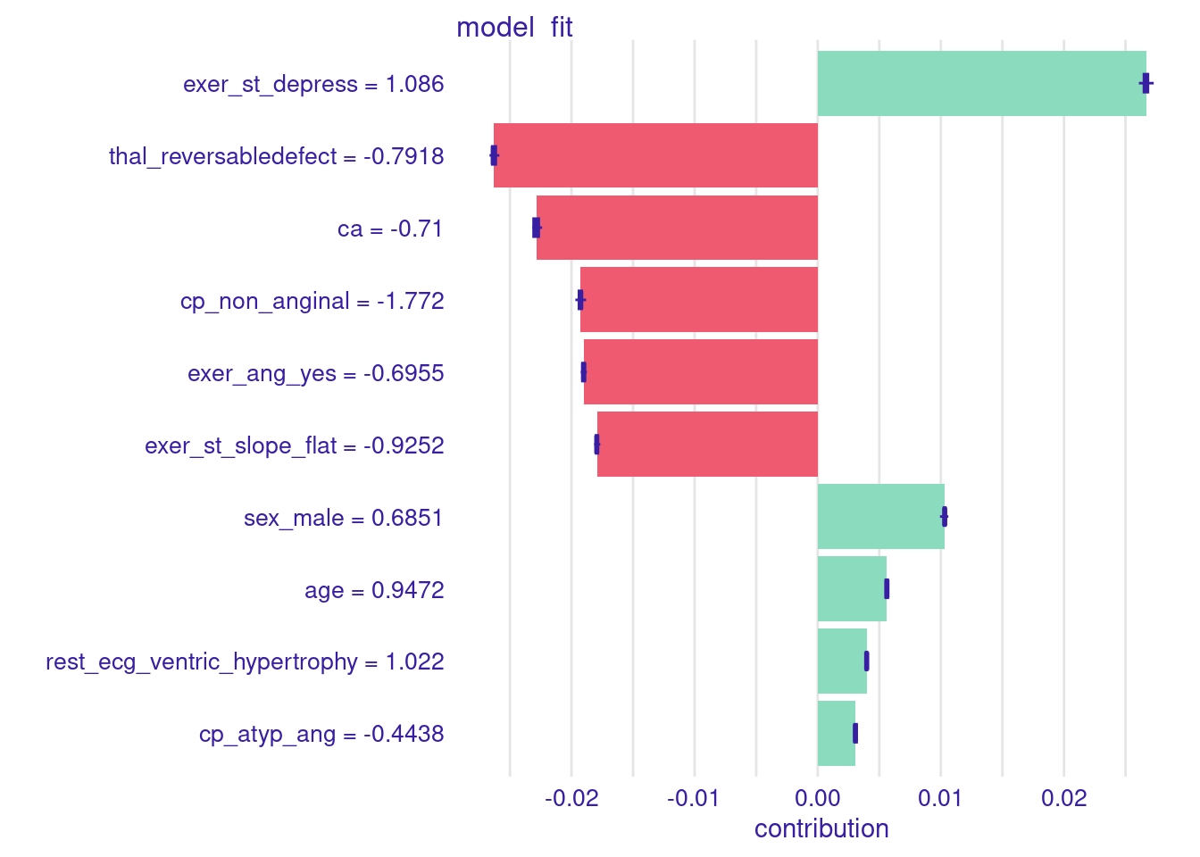

We can use these Shapley values for the local importance of the features for each observation to calculate the global importance of these features.

Features that have big absolute Shapley values on average across observation are more important. Let’s calculate this.

First we need a function to get shapley values for each observation (along with the feature values for a nicer plot)

get_shaps <- function(df1){
  predict_parts(explain_full, 
                new_observation = df1,
                type = "shap",
                B = 25) |> 
    filter(B == 0) |> 
    select(variable_name, variable_value, contribution) |> 
    as_tibble()
}

And then we can map this function over observations to get the Shapley values for each observation

local_shaps <- cache_rds(
  expr = {
    x |>
      slice_sample(prop = 1/5) |> # take random sample to reduce computation time
      mutate(id = row_number()) |>
      nest(.by = id, .key = "dfs") |>   # nest a dataframe for each observation
      mutate(shaps = map(dfs, \(df1) get_shaps(df1))) |> 
      select(-dfs) |>
      unnest(shaps)
  },
  rerun = rerun_setting,
  dir = "cache/011/",
  file = "local_shaps")

Here is what we get from applying the function over observations

local_shaps |> head()

# A tibble: 6 × 4
     id variable_name  variable_value contribution
  <int> <chr>          <chr>                 <dbl>
1     1 age            1.058               0.00626
2     1 ca             -0.71              -0.0229 
3     1 chol           1.281               0      
4     1 cp_atyp_ang    -0.4438             0.00308
5     1 cp_non_anginal 0.5624              0.00598
6     1 exer_ang_yes   -0.6955            -0.0190

Programming note: This code demonstrates another nice R programming technique using nest() and unnest() in combination with map() and list-columns. For more info, see this chapter in Wickham, Çetinkaya-Rundel, and Grolemund (2023) and the vignette on nesting (vignette("nest")).

Now that we have Shapley values for all observations, we can calculate the mean absolute Shapley value across observations and plot it.

Across all observations, ca contributes to an average change of .06 from the mean predicted probability of disease.
One of the features from our exercise test, exer_ang_yes, contributes about .05 change from mean predicted probability of disease.
The other exer_ features are not far behind.

local_shaps |>
  mutate(contribution = abs(contribution)) |>
  group_by(variable_name) |>
  summarize(mean_shap = mean(contribution)) |>
  arrange(desc(mean_shap)) |>
  mutate(variable_name = factor(variable_name),
         variable_name = fct_reorder(variable_name, mean_shap)) |>
  ggplot(aes(x = variable_name, y = mean_shap)) +
  geom_point() +
  coord_flip()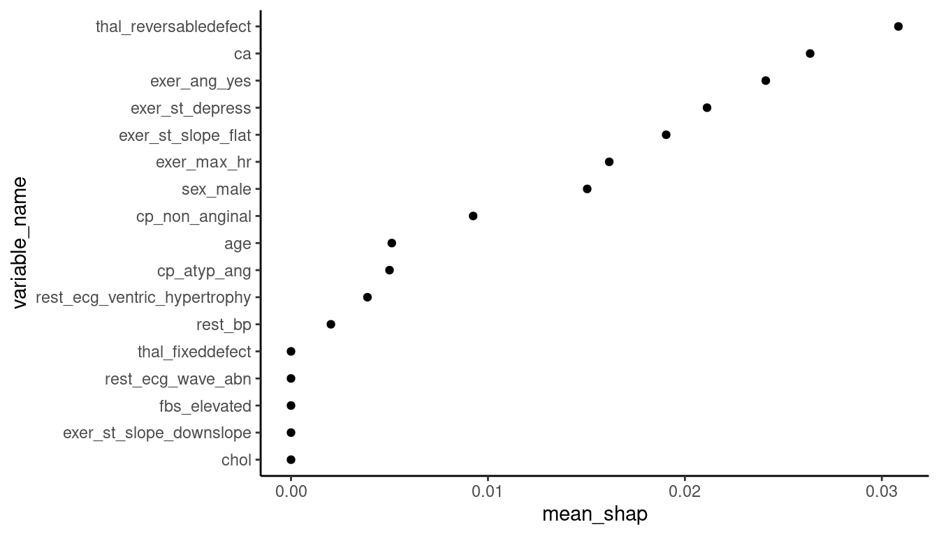

For a more advanced plot (a sina plot; not displayed here) we could superimpose the individual local Shapley values and color them based on the feature score.

This would allow us to show the direction of the relationship between the Shapley values and feature values.

See FIGURE 9.26 in Molnar (2023) for an example of this type of plot.

Shapley values are attractive relative to other approaches because

They have a solid theoretical basis
Sound statistical properties (Efficiency, Symmetry, Dummy and Additivity - see Molnar (2023))
Can provided a unified perspective across both local and global importance.

However, they can be VERY time consuming to calculate (particularly if you want to use them for global importance such that you need them for all/many observations).

There are computational shortcuts available but even those can be very time consuming in some instances (though XGBoost has a very fast implementation that we use regularly).

(Note that for decision tree based algorithms SHAP provides a more computationally efficient way to estimate Shapley values - see section 9.6 in Molnar (2023) for more detail.)

11.9 Visual Approaches to Understand our Models

We can also learn about how our features are used to make predictions in our models using visual approaches.

There are two key plots that we can use:

Partial Dependence (PD) Plots
Accumulated Local Effects (ALE) Plots

11.9.1 Partial Dependence (PD) Plots

The Partial dependence (PD) plot displays the marginal effect of a target feature or combination of features on the predictions from a model.

In essence, the prediction for any value of a target feature is the average prediction across cases if we set all cases to have that value for the target feature but their observed values for all other features.

We can use PD plots to understand whether the relationship between a target feature and the outcome is linear, monotonic, or more complex. It may also help us visualize and understand if interactions between features exist (if we make a PD plot for two target features).

The PD Plot is attractive because

it is easy to understand (prediction for each feature value averaged across observed values for all other features)
if the target feature is uncorrelated with all other features, its interpretation is clear, it is how the average prediction changes as the target features changes values.
it is computationally easy to implement
it has a causal (for the model, not the real world!) interpretation. This is what happens to the predciction if we manipulate the values of the target feature but hold all other features constant at their observed values.

However:

The assumption that the target feature is not correlated with the other features is likely unrealistic in many/most instances
This plot (but also other plot methods) are limited to 1 - 2 features in combination.
It may hide effects when interactions exist

11.9.2 Accumulated Local Effects (ALE) Plots

If the features are correlated, the partial dependence plot should not be used because the plots will otherwise be based on combinations of the target feature and other features that may never occur (given the feature correlations).

Molnar describes how this problem of correlated features and unrealistic combinations of features can be solved by M-Plots that plot the average effect of a target feature using the conditional values on other features (i.e., only using realistic values for the other features based on their correlations with the target feature). Unfortunately, this too is sub-optimal because it will confound the effect of the target feature with the effects of the other features that are correlated with it.

Accumulated Local Effects (ALE) plots also use conditional values of other features to solve the correlated features problem. However, ALE plots solve the confounding problem by calculating differences in predictions associated with changes in the target feature rather than average predictions for each value of that target feature. These differences hold the other features values (mostly) constant to remove their effects.

ALE plots are the preferred plot in situations where you expect your target feature to be correlated with other features (which is likely most situations.)

We will use the DALEX package again to make these PD and ALE plots.

It will require the explainer object we created earlier for feature importance

Otherwise, the code is very straight-forward. Here we get the predicted values for an ALE plot to examine the effect of one of the features from our exercise test (exer_max_hr) on disease probabilities.

If we wanted a PD plot, we could simply substitute partial for accumulated

ale <- model_profile(explainer = explain_full,
                     type = "accumulated",
                     variables = "exer_max_hr",
                     N = NULL)  # to use full sample (default is 100)

There is a default plot function for these plot object (or you could use the data in the object to make your own ggplot)

The probability of disease decreases as max hr increases in the exercise test

ale |> plot()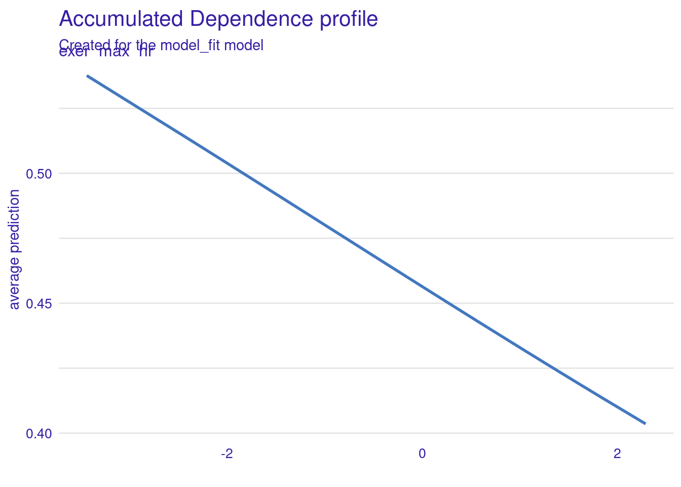

11.10 Summary and Closing Thoughts

When pursuing purely explanatory goals with machine learning methods, we can:

Use resampling with the full dataset to determine appropriate model configuration
- Best statistical algorithm
- Which covariates
- Other “researcher degrees of freedom” such as handling of outliers, transformations of predictors
Use model comparisons (Frequentist or Bayesian) in combination with feature ablation to test effect of feature or set of features
We can use feature importance measures (permutation or Shapley) to understand the contributions that various features make to prediction for an observation (local) or across observations (global)
We can explore the shape (and magnitude?) of relationships using PD and ALE plots

11.11 Discussion

11.11.1 Neural Net Winners

11.11.2 Permutation Test (quiz question 5 was updated so everyone got a point!)

Real quick though what is permutation?

It involves shuffling (permuting) the data many times.
After each permutation you refit the model and get a test-statistic (e.g., accuracy).
Essentially any relationship between features and the outcome are gone. So the permuted test-statistic is what we should expect to get if our features calculated no signal.
Then you would calculate the proportion of permutations where the test statistic is greater than or equal to your model performance estimate with the un-imputed data.
If this is below .05 your interpretation would be to reject NULL (i.e., your model is performing better than a model with no signal)

Example from ChatGPT of when a permutation test can come in hand:

Imagine you have two groups of people, and you want to see if there’s a difference in their average heights. You measure everyone, and you find that, on average, Group A is taller than Group B. But you wonder: Is this difference just due to random chance, or is there something real going on?

It also doesn’t have any assumption requirements for your data

But…It is computationally expensive and there are often other more efficient methods for testing your model’s performance.

11.11.3 Ice Breaker

Get into pairs or small groups. Think about one of the data sets we have worked with in class or your own! Create a research question you might ask using each of the following explanatory methods.

Permutation
Bayesian model comparison
Shapley values

11.11.4 Question 5 from quiz

Let’s say you want to build a model to predict which individuals will develop hypertension based on health data within patients’ medical records (e.g. family history, medical chart notes, genetic testing results). Which of the following claims about your model could be investigated using a permutation test?

Addition of genetic data to our model does not significantly improve upon the accuracy of models using only family history and medical chart notes
Family history variables are more important for prediction of future hypertension than medical chart notes
The predictors from patients’ medical records are related to their hypertension and your model is capturing this relationship to some degree
Our model performs significantly better than leading diagnostic screening questionnaires for prediction of future hypertension

What method would we use to investigate the other claims?

11.11.5 Question 3 from quiz

Imagine you want to determine if an elastic net logistic regression model (that you tuned on penalty and mixture) is performing better than would be expected by chance. Which situations would require you to include the model selection process inside of your permutation test? Select all that apply.

Model selection was performed via k-fold cross validation, model evaluation was performed in an independent test set b. Model selection and evaluation was performed via bootstrapped resampling
Model selection and evaluation was performed via nested resampling
You always need to include model selection processes inside of permutation tests

Why not the other methods?

11.11.6 Bayesian Model Comparisons

Conceptually - could we go over posterior probabilities again - I was a bit confused on what this is and how that differ from other metrics that we use.
Posterior probabilities are a way for us to estimate the likelihood of a parameter being a certain value. For example, the probability that are model is performing within a certain range (e.g., how probable various values are for the accuracy of each model).

Whereas before we used resampling to obtain performance estimates of our model and stopped there. Now we can use these estimates as data to pass into perf_mod() an get a distribution of probabilities that the true performance estimate falls within a certain range.

What do HDI values represent?
The range of parameter estimate values that include 95% of the credible values.

Lets look at an example figure.

Is the probability that full model is better than compact model deemed as ‘p-value’ in Bayesian way? What’s the difference between using a ROPE to inspect on the result and using a p-value?

https://jjcurtin.github.io/book_iaml/011_explanation.html#bayesian-estimation-for-model-comparisons

11.11.7 Shapley Values

I feel like I dont have a good grasp on Shapely values.What do they really mean and how are they interpreted

Shapley values give us a measure of relative feature importance (i.e., which features are contributing most to a model’s predictions compared to other features). For classification models, Shapley values represent the impact of each feature on the probability of the predicted class.

They are calculated by considering all the possible ways features can be ordered in a model. Then, for each possible ordering, the contribution of each feature is measured when an additional feature is added. Finally, the contribution of each feature is averaged across all possible orders. This is why it took so long to run in your homework assignment!

So, how do we know which features are most important? How might we report our findings about top features?

We look at the relative ordering of features and the ones with the highest Shapley value are the most important for our model’s predictions. We can use the Shapley value to indicate how much each feature contributes to the change in probability of our positive class being predicted.

Note Shapley values are not inferential tests, they are descriptive!

Can you talk more about Shapley values (SHAP), as well as local importance and global importance?

Anyone want to volunteer to explain the difference?

What is a real-life example of some data where we might care about feature importance?

Lets look at an example from John’s lab!

Additivity principle of Shapley values

The difference between permutation feature importance and shapley values.

Permutation feature importance focuses on how shuffling a feature’s values affects the model’s overall performance (i.e., removing any association between the feature and outcome), while Shapley values focus on the marginal contribution of each feature to individual predictions.

When using L1 and L2 penalties, does it use feature importance to decide which features to drop out/down?

Lasso and Ridge penalties shrink the coefficients of less important features, but does so by adding a penalty to the loss function. This is different than calculating feature importance with permutation or Shapley methods. Remember penalties are for reducing overfitting of a model, and indices of feature importance are for explaining the output of a model.

Benavoli, Alessio, Giorgio Coraniy, Janez Demsar, and Marco Zaffalon. 2017. “Time for a Change: A Tutorial for Comparing Multiple Classifiers Through Bayesian Analysis.” Journal of Machine Learning Research 18: 1–36.

Bouckaert, Remco R. 2003. “Choosing Between Two Learning Algorithms Based on Calibrated Tests.” In Proceedings of the Twentieth International Conference on International Conference on Machine Learning, 51–58. ICML’03. Washington, DC, USA: AAAI Press.

Kruschke, John K. 2018. “Rejecting or Accepting Parameter Values in Bayesian Estimation.” Advances in Methods and Practices in Psychological Science 1: 270–80.

Molnar, Christoph. 2023. Intepretable Machine Learning: A Guide for Makiong Black Box MOdels Explainable. 2nd ed. https://christophm.github.io/interpretable-ml-book/.

Nadeau, Claude, and Yoshua Bengio. 2003. “Inference for the Generalization Error.” Machine Learning 52 (3): 239–81. https://doi.org/10.1023/A:1024068626366.

Wickham, Hadley, Çetinkaya-Rundel Mine, and Garrett Grolemund. 2023. R for Data Science: Visualize, Model, Transform, and Import Data. 2nd ed. https://r4ds.hadley.nz/.