NOTES: Please read the above chapters more with an eye toward concepts and issues rather than code. I will demonstrate a minimum set of functions to accomplish the NLP modeling tasks for this unit.
Also know that the entire Hvitfeldt and Silge (2022, book) is really mandatory reading. I would also strongly recommend this entire Silge and Robinson (2017)book. Both will be important references at a minimum.
8 str_split(x, pattern) splits up a string into multiple pieces.
str_split(c("a,b", "c,d,e"), ",")
[[1]]
[1] "a" "b"

[[2]]
[1] "c" "d" "e"
12.2.2 Regular Expressions
Regular expressions are a way to specify or search for patterns of strings using a sequence of characters. By combining a selection of simple patterns, we can capture quite complicated strings.
The stringr package uses regular expressions extensively
The regular expressions are passed as the pattern = argument. Regular expressions can be used to detect, locate, or extract parts of a string.
Julia Silge has put together a wonderful tutorial/primer on the use of regular expressions. After reading it, I finally had a solid grasp on them. Rather than grab sections, I will direct you to it (and review it live in our filmed lectures). She does it much better than I could!
You might consider installing the RegExplainpackage using devtools if you want more support working with regular expressions. They are powerful but they are complicated to learn initially
There is also a very helpful cheatsheet for regular expressions
And finally, there is a great Wickham, Çetinkaya-Rundel, and Grolemund (2023) chapter on strings more generally, which covers both stringr and regex.
12.3 The IMDB Dataset
Now that we have a basic understanding of how to manipulation raw text, we can get set up for NLP and introduce a guiding example for this unit
We can start with our normal cast of characters RE packages, source, and settings (not displayed here)
However, we will also install a few new ones that are specific to working with text.
library(tidytext)library(textrecipes) #step_- functions for NLPlibrary(SnowballC) library(stopwords)
The IMDB Reviews dataset is a classic NLP dataset that is used for sentiment analysis
It contains:
25,000 movie reviews in train and test
Balanced on positive and negative sentiment (labeled outcome)
Story of a man who has unnatural feelings for a pig. Starts out with a opening scene that is a terrific example of absurd comedy. A formal orchestra audience is turned into an insane, violent mob by the crazy chantings of it's singers. Unfortunately it stays absurd the WHOLE time with no general narrative eventually making it just too off putting. Even those from the era should be turned off. The cryptic dialogue would make Shakespeare seem easy to a third grader. On a technical level it's better than you might think with some good cinematography by future great Vilmos Zsigmond. Future stars Sally Kirkland and Frederic Forrest can be seen briefly.
Airport '77 starts as a brand new luxury 747 plane is loaded up with valuable paintings & such belonging to rich businessman Philip Stevens (James Stewart) who is flying them & a bunch of VIP's to his estate in preparation of it being opened to the public as a museum, also on board is Stevens daughter Julie (Kathleen Quinlan) & her son. The luxury jetliner takes off as planned but mid-air the plane is hi-jacked by the co-pilot Chambers (Robert Foxworth) & his two accomplice's Banker (Monte Markham) & Wilson (Michael Pataki) who knock the passengers & crew out with sleeping gas, they plan to steal the valuable cargo & land on a disused plane strip on an isolated island but while making his descent Chambers almost hits an oil rig in the Ocean & loses control of the plane sending it crashing into the sea where it sinks to the bottom right bang in the middle of the Bermuda Triangle. With air in short supply, water leaking in & having flown over 200 miles off course the problems mount for the survivor's as they await help with time fast running out...<br /><br />Also known under the slightly different tile Airport 1977 this second sequel to the smash-hit disaster thriller Airport (1970) was directed by Jerry Jameson & while once again like it's predecessors I can't say Airport '77 is any sort of forgotten classic it is entertaining although not necessarily for the right reasons. Out of the three Airport films I have seen so far I actually liked this one the best, just. It has my favourite plot of the three with a nice mid-air hi-jacking & then the crashing (didn't he see the oil rig?) & sinking of the 747 (maybe the makers were trying to cross the original Airport with another popular disaster flick of the period The Poseidon Adventure (1972)) & submerged is where it stays until the end with a stark dilemma facing those trapped inside, either suffocate when the air runs out or drown as the 747 floods or if any of the doors are opened & it's a decent idea that could have made for a great little disaster flick but bad unsympathetic character's, dull dialogue, lethargic set-pieces & a real lack of danger or suspense or tension means this is a missed opportunity. While the rather sluggish plot keeps one entertained for 108 odd minutes not that much happens after the plane sinks & there's not as much urgency as I thought there should have been. Even when the Navy become involved things don't pick up that much with a few shots of huge ships & helicopters flying about but there's just something lacking here. George Kennedy as the jinxed airline worker Joe Patroni is back but only gets a couple of scenes & barely even says anything preferring to just look worried in the background.<br /><br />The home video & theatrical version of Airport '77 run 108 minutes while the US TV versions add an extra hour of footage including a new opening credits sequence, many more scenes with George Kennedy as Patroni, flashbacks to flesh out character's, longer rescue scenes & the discovery or another couple of dead bodies including the navigator. While I would like to see this extra footage I am not sure I could sit through a near three hour cut of Airport '77. As expected the film has dated badly with horrible fashions & interior design choices, I will say no more other than the toy plane model effects aren't great either. Along with the other two Airport sequels this takes pride of place in the Razzie Award's Hall of Shame although I can think of lots of worse films than this so I reckon that's a little harsh. The action scenes are a little dull unfortunately, the pace is slow & not much excitement or tension is generated which is a shame as I reckon this could have been a pretty good film if made properly.<br /><br />The production values are alright if nothing spectacular. The acting isn't great, two time Oscar winner Jack Lemmon has said since it was a mistake to star in this, one time Oscar winner James Stewart looks old & frail, also one time Oscar winner Lee Grant looks drunk while Sir Christopher Lee is given little to do & there are plenty of other familiar faces to look out for too.<br /><br />Airport '77 is the most disaster orientated of the three Airport films so far & I liked the ideas behind it even if they were a bit silly, the production & bland direction doesn't help though & a film about a sunken plane just shouldn't be this boring or lethargic. Followed by The Concorde ... Airport '79 (1979).
This film lacked something I couldn't put my finger on at first: charisma on the part of the leading actress. This inevitably translated to lack of chemistry when she shared the screen with her leading man. Even the romantic scenes came across as being merely the actors at play. It could very well have been the director who miscalculated what he needed from the actors. I just don't know.<br /><br />But could it have been the screenplay? Just exactly who was the chef in love with? He seemed more enamored of his culinary skills and restaurant, and ultimately of himself and his youthful exploits, than of anybody or anything else. He never convinced me he was in love with the princess.<br /><br />I was disappointed in this movie. But, don't forget it was nominated for an Oscar, so judge for yourself.
Sorry everyone,,, I know this is supposed to be an "art" film,, but wow, they should have handed out guns at the screening so people could blow their brains out and not watch. Although the scene design and photographic direction was excellent, this story is too painful to watch. The absence of a sound track was brutal. The loooonnnnng shots were too long. How long can you watch two people just sitting there and talking? Especially when the dialogue is two people complaining. I really had a hard time just getting through this film. The performances were excellent, but how much of that dark, sombre, uninspired, stuff can you take? The only thing i liked was Maureen Stapleton and her red dress and dancing scene. Otherwise this was a ripoff of Bergman. And i'm no fan f his either. I think anyone who says they enjoyed 1 1/2 hours of this is,, well, lying.
When I was little my parents took me along to the theater to see Interiors. It was one of many movies I watched with my parents, but this was the only one we walked out of. Since then I had never seen Interiors until just recently, and I could have lived out the rest of my life without it. What a pretentious, ponderous, and painfully boring piece of 70's wine and cheese tripe. Woody Allen is one of my favorite directors but Interiors is by far the worst piece of crap of his career. In the unmistakable style of Ingmar Berman, Allen gives us a dark, angular, muted, insight in to the lives of a family wrought by the psychological damage caused by divorce, estrangement, career, love, non-love, halitosis, whatever. The film, intentionally, has no comic relief, no music, and is drenched in shadowy pathos. This film style can be best defined as expressionist in nature, using an improvisational method of dialogue to illicit a "more pronounced depth of meaning and truth". But Woody Allen is no Ingmar Bergman. The film is painfully slow and dull. But beyond that, I simply had no connection with or sympathy for any of the characters. Instead I felt only contempt for this parade of shuffling, whining, nicotine stained, martyrs in a perpetual quest for identity. Amid a backdrop of cosmopolitan affluence and baked Brie intelligentsia the story looms like a fart in the room. Everyone speaks in affected platitudes and elevated language between cigarettes. Everyone is "lost" and "struggling", desperate to find direction or understanding or whatever and it just goes on and on to the point where you just want to slap all of them. It's never about resolution, it's only about interminable introspective babble. It is nothing more than a psychological drama taken to an extreme beyond the audience's ability to connect. Woody Allen chose to make characters so immersed in themselves we feel left out. And for that reason I found this movie painfully self indulgent and spiritually draining. I see what he was going for but his insistence on promoting his message through Prozac prose and distorted film techniques jettisons it past the point of relevance. I highly recommend this one if you're feeling a little too happy and need something to remind you of death. Otherwise, let's just pretend this film never happened.
and the first five positive reviews from the training set
Bromwell High is a cartoon comedy. It ran at the same time as some other programs about school life, such as "Teachers". My 35 years in the teaching profession lead me to believe that Bromwell High's satire is much closer to reality than is "Teachers". The scramble to survive financially, the insightful students who can see right through their pathetic teachers' pomp, the pettiness of the whole situation, all remind me of the schools I knew and their students. When I saw the episode in which a student repeatedly tried to burn down the school, I immediately recalled ......... at .......... High. A classic line: INSPECTOR: I'm here to sack one of your teachers. STUDENT: Welcome to Bromwell High. I expect that many adults of my age think that Bromwell High is far fetched. What a pity that it isn't!
Homelessness (or Houselessness as George Carlin stated) has been an issue for years but never a plan to help those on the street that were once considered human who did everything from going to school, work, or vote for the matter. Most people think of the homeless as just a lost cause while worrying about things such as racism, the war on Iraq, pressuring kids to succeed, technology, the elections, inflation, or worrying if they'll be next to end up on the streets.<br /><br />But what if you were given a bet to live on the streets for a month without the luxuries you once had from a home, the entertainment sets, a bathroom, pictures on the wall, a computer, and everything you once treasure to see what it's like to be homeless? That is Goddard Bolt's lesson.<br /><br />Mel Brooks (who directs) who stars as Bolt plays a rich man who has everything in the world until deciding to make a bet with a sissy rival (Jeffery Tambor) to see if he can live in the streets for thirty days without the luxuries; if Bolt succeeds, he can do what he wants with a future project of making more buildings. The bet's on where Bolt is thrown on the street with a bracelet on his leg to monitor his every move where he can't step off the sidewalk. He's given the nickname Pepto by a vagrant after it's written on his forehead where Bolt meets other characters including a woman by the name of Molly (Lesley Ann Warren) an ex-dancer who got divorce before losing her home, and her pals Sailor (Howard Morris) and Fumes (Teddy Wilson) who are already used to the streets. They're survivors. Bolt isn't. He's not used to reaching mutual agreements like he once did when being rich where it's fight or flight, kill or be killed.<br /><br />While the love connection between Molly and Bolt wasn't necessary to plot, I found "Life Stinks" to be one of Mel Brooks' observant films where prior to being a comedy, it shows a tender side compared to his slapstick work such as Blazing Saddles, Young Frankenstein, or Spaceballs for the matter, to show what it's like having something valuable before losing it the next day or on the other hand making a stupid bet like all rich people do when they don't know what to do with their money. Maybe they should give it to the homeless instead of using it like Monopoly money.<br /><br />Or maybe this film will inspire you to help others.
Brilliant over-acting by Lesley Ann Warren. Best dramatic hobo lady I have ever seen, and love scenes in clothes warehouse are second to none. The corn on face is a classic, as good as anything in Blazing Saddles. The take on lawyers is also superb. After being accused of being a turncoat, selling out his boss, and being dishonest the lawyer of Pepto Bolt shrugs indifferently "I'm a lawyer" he says. Three funny words. Jeffrey Tambor, a favorite from the later Larry Sanders show, is fantastic here too as a mad millionaire who wants to crush the ghetto. His character is more malevolent than usual. The hospital scene, and the scene where the homeless invade a demolition site, are all-time classics. Look for the legs scene and the two big diggers fighting (one bleeds). This movie gets better each time I see it (which is quite often).
This is easily the most underrated film inn the Brooks cannon. Sure, its flawed. It does not give a realistic view of homelessness (unlike, say, how Citizen Kane gave a realistic view of lounge singers, or Titanic gave a realistic view of Italians YOU IDIOTS). Many of the jokes fall flat. But still, this film is very lovable in a way many comedies are not, and to pull that off in a story about some of the most traditionally reviled members of society is truly impressive. Its not The Fisher King, but its not crap, either. My only complaint is that Brooks should have cast someone else in the lead (I love Mel as a Director and Writer, not so much as a lead).
This is not the typical Mel Brooks film. It was much less slapstick than most of his movies and actually had a plot that was followable. Leslie Ann Warren made the movie, she is such a fantastic, under-rated actress. There were some moments that could have been fleshed out a bit more, and some scenes that could probably have been cut to make the room to do so, but all in all, this is worth the price to rent and see it. The acting was good overall, Brooks himself did a good job without his characteristic speaking to directly to the audience. Again, Warren was the best actor in the movie, but "Fume" and "Sailor" both played their parts well.
You need to spend a LOT of time reviewing the text before you begin to process it.
I have NOT done this yet!
My models will be sub-optimal!
12.4 Tokens
Machine learning algorithms cannot work with raw text (documents) directly
We must feature engineer these documents to allow them to serve as input to statistical algorithms
The first step for most NLP feature engineering methods is to represent text (documents) as tokens (words, ngrams)
Given that tokenization is often one of our first steps for extracting features from text, it is important to consider carefully what happens during this step and its implications for your subsequent modeling
In tokenization, we take input documents (text strings) and a token type (a meaningful unit of text, such as a word) and split the document into pieces (tokens) that correspond to the type
We can tokenize text into a variety of token types:
characters
words (most common - our focus; unigrams)
sentences
lines
paragraphs
n-grams (bigrams, trigrams)
An n-gram consists of a sequence of n items from a given sequence of text. Most often, it is a group of n words (bigrams, trigrams)
n-grams retain word order which would otherwise be lost if we were just using words as the token type
“I am not happy”
Tokenized by word, yields:
I
am
not
happy
Tokenized by 2-gram words:
I am
am not
not happy
We will be using tokenizer functions from the tokenizers package. Three in particular are:
However, we will be accessing these functions through wrappers:
tidytext::unnest_tokens(tbl, output, input, token = "words", format = c("text", "man", "latex", "html", "xml"), to_lower = TRUE, drop = TRUE, collapse = NULL) for tidyverse data exploration of tokens within tibbles
textrecipes::step_tokenize() for tokenization in our recipes
Word-level tokenization by tokenize_words() is done by finding word boundaries as follows:
Break at the start and end of text, unless the text is empty
Do not break within CRLF (new line characters)
Otherwise, break before and after new lines (including CR and LF)
Do not break between most letters
Do not break letters across certain punctuation
Do not break within sequences of digits, or digits adjacent to letters (“3a,” or “A3”)
Do not break within sequences, such as “3.2” or “3,456.789.”
Do not break between Katakana
Do not break from extenders
Do not break within emoji zwj sequences
Do not break within emoji flag sequences
Ignore Format and Extend characters, except after sot, CR, LF, and new line
Keep horizontal whitespace together
Otherwise, break everywhere (including around ideographs, e.g., @, %, >)
Let’s start with using tokenize_words() to get a sense of how it works by default
Splits on spaces
Converts to lowercase by default (does it matter? MAYBE!!!)
Retains apostrophes but drops other punctuation (,, ., !) and some symbols (e.g., -\\, @) by default. Does not drop _ (Do you need punctuation? !!!!)
Retains numbers (by default) and decimals but drops + appended to 4+
Has trouble with URLs and email address (do you need this?)
Often, these issues may NOT matter
"Here is a sample document to tokenize. How EXCITING (I _love_ it). Sarah has spent 4 or 4.1 or 4P or 4+ or >4 years developing her pre-processing and NLP skills. You can learn more about tokenization here: https://smltar.com/tokenization.html or by emailing me at jjcurtin@wisc.edu"|> tokenizers::tokenize_words()
Some of these behaviors can be altered from their defaults
lowercase = TRUE
strip_punc = TRUE
strip_numeric = FALSE
Some of these issues can be corrected by pre-processing the text
str_replace("jjcurtin@wisc.edu", "@", "_at_")
[1] "jjcurtin_at_wisc.edu"
If you need finer control, you can use tokenize_regex() and then do further processing with stringr functions and regex
Now it may be easier to build up from here (e.g., ):
str_to_lower(word)
str_replace(word, ".$", "")
"Here is a sample document to tokenize. How EXCITING (I _love_ it). Sarah has spent 4 or 4.1 or 4P or 4+ years developing her pre-processing and NLP skills. You can learn more about tokenization here: https://smltar.com/tokenization.html or by emailing me at jjcurtin@wisc.edu"|> tokenizers::tokenize_regex(pattern ="\\s+")
You can explore the tokens that will be formed using unnest_tokens() and basic tidyverse data wrangling using a tidied format of your documents as part of your EDA
We unnest to 1 token (word) per row (tidy format)
We keep track of doc_num (added earlier)
Here, we tokenize the IMDB training set.
Using defaults
Can change other default for tokenize_*() by passing into function via ...
Can set drop = TRUE (default) to discard the original document column (text)
Rows: 5,935,548
Columns: 4
$ doc_num   <int> 1, 1, 1, 1, 1, 1, 1, 1, 1, 1, 1, 1, 1, 1, 1, 1, 1, 1, 1, 1, …
$ sentiment <fct> neg, neg, neg, neg, neg, neg, neg, neg, neg, neg, neg, neg, …
$ text      <chr> "Story of a man who has unnatural feelings for a pig. Starts…
$ word      <chr> "story", "of", "a", "man", "who", "has", "unnatural", "feeli…
Coding sidebar: You can take a much deeper dive into tidyverse text processing in chapter 1 of Silge and Robinson (2017).
Let’s get oriented by reviewing the tokens from the first document
Raw form
data_trn$text[1]
[1] "Story of a man who has unnatural feelings for a pig. Starts out with a opening scene that is a terrific example of absurd comedy. A formal orchestra audience is turned into an insane, violent mob by the crazy chantings of it's singers. Unfortunately it stays absurd the WHOLE time with no general narrative eventually making it just too off putting. Even those from the era should be turned off. The cryptic dialogue would make Shakespeare seem easy to a third grader. On a technical level it's better than you might think with some good cinematography by future great Vilmos Zsigmond. Future stars Sally Kirkland and Frederic Forrest can be seen briefly."
# A tibble: 112 × 1
    word
    <chr>
  1 story
  2 of
  3 a
  4 man
  5 who
  6 has
  7 unnatural
  8 feelings
  9 for
 10 a
 11 pig
 12 starts
 13 out
 14 with
 15 a
 16 opening
 17 scene
 18 that
 19 is
 20 a
 21 terrific
 22 example
 23 of
 24 absurd
 25 comedy
 26 a
 27 formal
 28 orchestra
 29 audience
 30 is
 31 turned
 32 into
 33 an
 34 insane
 35 violent
 36 mob
 37 by
 38 the
 39 crazy
 40 chantings
 41 of
 42 it's
 43 singers
 44 unfortunately
 45 it
 46 stays
 47 absurd
 48 the
 49 whole
 50 time
 51 with
 52 no
 53 general
 54 narrative
 55 eventually
 56 making
 57 it
 58 just
 59 too
 60 off
 61 putting
 62 even
 63 those
 64 from
 65 the
 66 era
 67 should
 68 be
 69 turned
 70 off
 71 the
 72 cryptic
 73 dialogue
 74 would
 75 make
 76 shakespeare
 77 seem
 78 easy
 79 to
 80 a
 81 third
 82 grader
 83 on
 84 a
 85 technical
 86 level
 87 it's
 88 better
 89 than
 90 you
 91 might
 92 think
 93 with
 94 some
 95 good
 96 cinematography
 97 by
 98 future
 99 great
100 vilmos
101 zsigmond
102 future
103 stars
104 sally
105 kirkland
106 and
107 frederic
108 forrest
109 can
110 be
111 seen
112 briefly
Considering all the tokens across all documents
There are almost 6 million words
length(tokens$word)
[1] 5935548
The total unique vocabulary is around 85 thousand words
length(unique(tokens$word))
[1] 85574
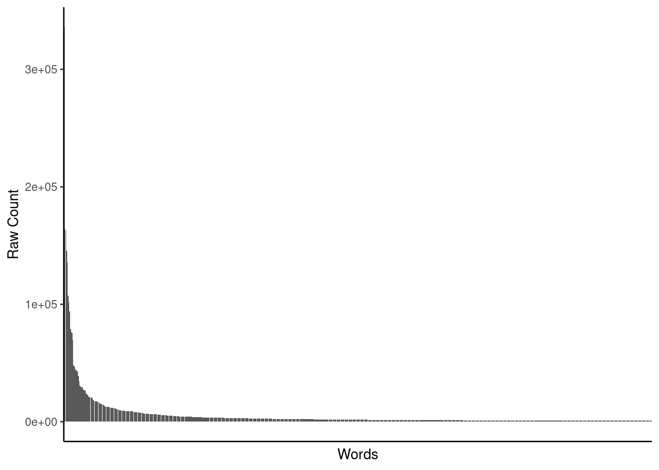
Word frequency is VERY skewed
These are the counts for the most frequent 750 words
there are 84,000 additional infrequent words in the right tail not shown here!
Some of our feature engineering approaches (e.g., BoW) will use the first 5K - 20K tokens
Some of our feature engineering approaches (e.g., word embeddings) may use ALL tokens
Some of these are likely not very informative (the, a, of, to, is). We will return to those words in a bit when we consider stopwords
Notice br. Why is it so common?
tokens |>count(word, sort =TRUE) |>print(n =100)
# A tibble: 85,574 × 2
    word         n
    <chr>    <int>
  1 the     336179
  2 and     164061
  3 a       162738
  4 of      145848
  5 to      135695
  6 is      107320
  7 br      101871
  8 in       93920
  9 it       78874
 10 i        76508
 11 this     75814
 12 that     69794
 13 was      48189
 14 as       46903
 15 for      44321
 16 with     44115
 17 movie    43509
 18 but      42531
 19 film     39058
 20 on       34185
 21 not      30608
 22 you      29886
 23 are      29431
 24 his      29352
 25 have     27725
 26 be       26947
 27 he       26894
 28 one      26502
 29 all      23927
 30 at       23500
 31 by       22538
 32 an       21550
 33 they     21096
 34 who      20604
 35 so       20573
 36 from     20488
 37 like     20268
 38 her      18399
 39 or       17997
 40 just     17764
 41 about    17368
 42 out      17099
 43 it's     17094
 44 has      16789
 45 if       16746
 46 some     15734
 47 there    15671
 48 what     15374
 49 good     15110
 50 more     14242
 51 when     14161
 52 very     14059
 53 up       13283
 54 no       12698
 55 time     12691
 56 even     12638
 57 she      12624
 58 my       12485
 59 would    12236
 60 which    12047
 61 story    11918
 62 only     11910
 63 really   11734
 64 see      11465
 65 their    11376
 66 had      11289
 67 can      11144
 68 were     10782
 69 me       10745
 70 well     10637
 71 than      9920
 72 we        9858
 73 much      9750
 74 bad       9292
 75 been      9287
 76 get       9279
 77 will      9195
 78 do        9159
 79 also      9130
 80 into      9109
 81 people    9107
 82 other     9083
 83 first     9054
 84 because   9045
 85 great     9033
 86 how       8870
 87 him       8865
 88 most      8775
 89 don't     8445
 90 made      8351
 91 its       8156
 92 then      8097
 93 make      8018
 94 way       8005
 95 them      7954
 96 too       7820
 97 could     7745
 98 any       7653
 99 movies    7648
100 after     7617
# ℹ 85,474 more rows
Here is the first document that has the br token in it.
[1] "Airport '77 starts as a brand new luxury 747 plane is loaded up with valuable paintings & such belonging to rich businessman Philip Stevens (James Stewart) who is flying them & a bunch of VIP's to his estate in preparation of it being opened to the public as a museum, also on board is Stevens daughter Julie (Kathleen Quinlan) & her son. The luxury jetliner takes off as planned but mid-air the plane is hi-jacked by the co-pilot Chambers (Robert Foxworth) & his two accomplice's Banker (Monte Markham) & Wilson (Michael Pataki) who knock the passengers & crew out with sleeping gas, they plan to steal the valuable cargo & land on a disused plane strip on an isolated island but while making his descent Chambers almost hits an oil rig in the Ocean & loses control of the plane sending it crashing into the sea where it sinks to the bottom right bang in the middle of the Bermuda Triangle. With air in short supply, water leaking in & having flown over 200 miles off course the problems mount for the survivor's as they await help with time fast running out...<br /><br />Also known under the slightly different tile Airport 1977 this second sequel to the smash-hit disaster thriller Airport (1970) was directed by Jerry Jameson & while once again like it's predecessors I can't say Airport '77 is any sort of forgotten classic it is entertaining although not necessarily for the right reasons. Out of the three Airport films I have seen so far I actually liked this one the best, just. It has my favourite plot of the three with a nice mid-air hi-jacking & then the crashing (didn't he see the oil rig?) & sinking of the 747 (maybe the makers were trying to cross the original Airport with another popular disaster flick of the period The Poseidon Adventure (1972)) & submerged is where it stays until the end with a stark dilemma facing those trapped inside, either suffocate when the air runs out or drown as the 747 floods or if any of the doors are opened & it's a decent idea that could have made for a great little disaster flick but bad unsympathetic character's, dull dialogue, lethargic set-pieces & a real lack of danger or suspense or tension means this is a missed opportunity. While the rather sluggish plot keeps one entertained for 108 odd minutes not that much happens after the plane sinks & there's not as much urgency as I thought there should have been. Even when the Navy become involved things don't pick up that much with a few shots of huge ships & helicopters flying about but there's just something lacking here. George Kennedy as the jinxed airline worker Joe Patroni is back but only gets a couple of scenes & barely even says anything preferring to just look worried in the background.<br /><br />The home video & theatrical version of Airport '77 run 108 minutes while the US TV versions add an extra hour of footage including a new opening credits sequence, many more scenes with George Kennedy as Patroni, flashbacks to flesh out character's, longer rescue scenes & the discovery or another couple of dead bodies including the navigator. While I would like to see this extra footage I am not sure I could sit through a near three hour cut of Airport '77. As expected the film has dated badly with horrible fashions & interior design choices, I will say no more other than the toy plane model effects aren't great either. Along with the other two Airport sequels this takes pride of place in the Razzie Award's Hall of Shame although I can think of lots of worse films than this so I reckon that's a little harsh. The action scenes are a little dull unfortunately, the pace is slow & not much excitement or tension is generated which is a shame as I reckon this could have been a pretty good film if made properly.<br /><br />The production values are alright if nothing spectacular. The acting isn't great, two time Oscar winner Jack Lemmon has said since it was a mistake to star in this, one time Oscar winner James Stewart looks old & frail, also one time Oscar winner Lee Grant looks drunk while Sir Christopher Lee is given little to do & there are plenty of other familiar faces to look out for too.<br /><br />Airport '77 is the most disaster orientated of the three Airport films so far & I liked the ideas behind it even if they were a bit silly, the production & bland direction doesn't help though & a film about a sunken plane just shouldn't be this boring or lethargic. Followed by The Concorde ... Airport '79 (1979)."
Let’s clean it in the raw documents and re-tokenize
You should always check your replacements CAREFULLY before doing them for unexpected matches and side-effects
We should continue to review MUCH deeper into the common tokens to detect other tokenization errors. I will not demonstrate that here.
We should also review the least common tokens
Worth searching to make sure they haven’t resulted from tokenization errors
Can use this to tune our pre-processing and tokenization
BUT, not as important b/c these will be dropped by some of our feature engineering approaches (BoW) and may not present too much problem to others (embeddings)
[1] "I am shocked. Shocked and dismayed that the 428 of you IMDB users who voted before me have not given this film a rating of higher than 7. 7?!?? - that's a C!. If I could give FOBH a 20, I'd gladly do it. This film ranks high atop the pantheon of modern comedy, alongside Half Baked and Mallrats, as one of the most hilarious films of all time. If you know _anything_ about rap music - YOU MUST SEE THIS!! If you know nothing about rap music - learn something!, and then see this! Comparisons to 'Spinal Tap' fail to appreciate the inspired genius of this unique film. If you liked Bob Roberts, you'll love this. Watch it and vote it a 10!"
[1] "Before I start, I _love_ Eddie Izzard. I think he's one of the funniest stand-ups around today. Possibly that means I'm going into this with too high expectations, but I just didn't find Eddie funny in this outing. I think the main problem is Eddie is trying too hard to be Eddie. Everyone knows him as a completely irrelevant comic, and we all love him for it. But in Circle, he appears to be going more for irrelevant than funny, and completely lost me in places. Many of the topics he covers he has covered before - I even think I recognised a few recycled jokes in there. If you buy the DVD you'll find a behind-the-scenes look at Eddie's tour (interesting in places, but not very funny), and a French language version of one of his shows. Die-hards will enjoy seeing Eddie in a different language, but subtitled comedy isn't very funny. If you're a fan of Eddie you've either got this already or you're going to buy it whatever I say. If you're just passing through, buy Glorious or Dressed to Kill - you won't be disappointed. With Circle, you probably will."
Let’s find all the tokens that start or end with _
The tokenizer didn’t get rid of numbers connected to text
How do we want to handle these?
Could add a space to make them two words?
We will leave them as is
Other issues?
Mis-spellings
Repeated letters for emphasize or effect?
Did caps matter (default tokenization was to convert to lowercase)?
Domain knowledge is useful here though multiple model configurations can be considered
strings of words that aren’t meaningful (“Welcome to Facebook”)
In the above workflow, we:
tokenize
review tokens for issues
clean raw text documents
re-tokenize
In some instances, it may be easier to clean the token and then put them back together
tokenize
review tokens for issues
clean tokens
recreate document
tokenize
If this latter workflow feels easier (i.e., easier to regex into a token than a document), we will need code to put the tokens back together into a document
Here is an example using the first three documents (`slice(1:3)1) and no cleaning
Tokenize
tokens <- data_trn |>slice(1:3) |>unnest_tokens(word, text, drop =FALSE,strip_numeric =TRUE)
Now we can do further cleaning with tokens
INSERT CLEANING CHUNKS HERE
Then put back together. Could also collapse into text_cln to retain original text column
and any other cleaning we could have done with the tokens along the way….
data_trn_cln |>pull(text) |>print_kbl()
x
story of a man who has unnatural feelings for a pig starts out with a opening scene that is a terrific example of absurd comedy a formal orchestra audience is turned into an insane violent mob by the crazy chantings of it's singers unfortunately it stays absurd the whole time with no general narrative eventually making it just too off putting even those from the era should be turned off the cryptic dialogue would make shakespeare seem easy to a third grader on a technical level it's better than you might think with some good cinematography by future great vilmos zsigmond future stars sally kirkland and frederic forrest can be seen briefly
airport starts as a brand new luxury plane is loaded up with valuable paintings such belonging to rich businessman philip stevens james stewart who is flying them a bunch of vip's to his estate in preparation of it being opened to the public as a museum also on board is stevens daughter julie kathleen quinlan her son the luxury jetliner takes off as planned but mid air the plane is hi jacked by the co pilot chambers robert foxworth his two accomplice's banker monte markham wilson michael pataki who knock the passengers crew out with sleeping gas they plan to steal the valuable cargo land on a disused plane strip on an isolated island but while making his descent chambers almost hits an oil rig in the ocean loses control of the plane sending it crashing into the sea where it sinks to the bottom right bang in the middle of the bermuda triangle with air in short supply water leaking in having flown over miles off course the problems mount for the survivor's as they await help with time fast running out also known under the slightly different tile airport this second sequel to the smash hit disaster thriller airport was directed by jerry jameson while once again like it's predecessors i can't say airport is any sort of forgotten classic it is entertaining although not necessarily for the right reasons out of the three airport films i have seen so far i actually liked this one the best just it has my favourite plot of the three with a nice mid air hi jacking then the crashing didn't he see the oil rig sinking of the maybe the makers were trying to cross the original airport with another popular disaster flick of the period the poseidon adventure submerged is where it stays until the end with a stark dilemma facing those trapped inside either suffocate when the air runs out or drown as the floods or if any of the doors are opened it's a decent idea that could have made for a great little disaster flick but bad unsympathetic character's dull dialogue lethargic set pieces a real lack of danger or suspense or tension means this is a missed opportunity while the rather sluggish plot keeps one entertained for odd minutes not that much happens after the plane sinks there's not as much urgency as i thought there should have been even when the navy become involved things don't pick up that much with a few shots of huge ships helicopters flying about but there's just something lacking here george kennedy as the jinxed airline worker joe patroni is back but only gets a couple of scenes barely even says anything preferring to just look worried in the background the home video theatrical version of airport run minutes while the us tv versions add an extra hour of footage including a new opening credits sequence many more scenes with george kennedy as patroni flashbacks to flesh out character's longer rescue scenes the discovery or another couple of dead bodies including the navigator while i would like to see this extra footage i am not sure i could sit through a near three hour cut of airport as expected the film has dated badly with horrible fashions interior design choices i will say no more other than the toy plane model effects aren't great either along with the other two airport sequels this takes pride of place in the razzie award's hall of shame although i can think of lots of worse films than this so i reckon that's a little harsh the action scenes are a little dull unfortunately the pace is slow not much excitement or tension is generated which is a shame as i reckon this could have been a pretty good film if made properly the production values are alright if nothing spectacular the acting isn't great two time oscar winner jack lemmon has said since it was a mistake to star in this one time oscar winner james stewart looks old frail also one time oscar winner lee grant looks drunk while sir christopher lee is given little to do there are plenty of other familiar faces to look out for too airport is the most disaster orientated of the three airport films so far i liked the ideas behind it even if they were a bit silly the production bland direction doesn't help though a film about a sunken plane just shouldn't be this boring or lethargic followed by the concorde airport
this film lacked something i couldn't put my finger on at first charisma on the part of the leading actress this inevitably translated to lack of chemistry when she shared the screen with her leading man even the romantic scenes came across as being merely the actors at play it could very well have been the director who miscalculated what he needed from the actors i just don't know but could it have been the screenplay just exactly who was the chef in love with he seemed more enamored of his culinary skills and restaurant and ultimately of himself and his youthful exploits than of anybody or anything else he never convinced me he was in love with the princess i was disappointed in this movie but don't forget it was nominated for an oscar so judge for yourself
12.5 Stop words
Not all words are equally informative or useful to our model depending on the nature of our problem
Very common words often may carry little or no meaningful information
These words are called stop words
It is common advice and practice to remove stop words for various NLP tasks
Notice some of the top most frequent words among our tokens from IMDB reviews
# A tibble: 84,392 × 2
    word         n
    <chr>    <int>
  1 the     336185
  2 and     164061
  3 a       162743
  4 of      145848
  5 to      135695
  6 is      107320
  7 in       93920
  8 it       78874
  9 i        76508
 10 this     75814
 11 that     69794
 12 was      48189
 13 as       46904
 14 for      44321
 15 with     44115
 16 movie    43509
 17 but      42531
 18 film     39058
 19 on       34185
 20 not      30608
 21 you      29886
 22 are      29431
 23 his      29352
 24 have     27725
 25 be       26947
 26 he       26894
 27 one      26502
 28 all      23927
 29 at       23500
 30 by       22539
 31 an       21550
 32 they     21096
 33 who      20604
 34 so       20573
 35 from     20488
 36 like     20268
 37 her      18399
 38 or       17997
 39 just     17764
 40 about    17368
 41 out      17099
 42 it's     17094
 43 has      16789
 44 if       16746
 45 some     15734
 46 there    15671
 47 what     15374
 48 good     15110
 49 more     14242
 50 when     14161
 51 very     14059
 52 up       13283
 53 no       12698
 54 time     12691
 55 even     12638
 56 she      12624
 57 my       12485
 58 would    12236
 59 which    12047
 60 story    11919
 61 only     11910
 62 really   11734
 63 see      11465
 64 their    11376
 65 had      11289
 66 can      11144
 67 were     10782
 68 me       10745
 69 well     10637
 70 than      9920
 71 we        9858
 72 much      9750
 73 bad       9292
 74 been      9287
 75 get       9279
 76 will      9195
 77 do        9159
 78 also      9130
 79 into      9109
 80 people    9107
 81 other     9083
 82 first     9054
 83 because   9045
 84 great     9033
 85 how       8870
 86 him       8865
 87 most      8775
 88 don't     8445
 89 made      8351
 90 its       8156
 91 then      8097
 92 make      8018
 93 way       8005
 94 them      7954
 95 too       7820
 96 could     7746
 97 any       7653
 98 movies    7648
 99 after     7617
100 think     7293
# ℹ 84,292 more rows
Stop words can have different roles in a corpus (a set of documents)
For our purposes, we generally care about two different types of stop words:
Global
Subject-specific
Global stop words almost always have very little value for our modeling goals
These are frequent words like “the”, “of” and “and” in English.
It is typically pretty safe to remove these and you can find them in pre-made lists of stop words (see below)
Subject-specific stop words are words that are common and uninformative given the subject or context within which your text/documents were collected and your modeling goals.
For example, given our goal to classify movie reviews as positive or negative, subject-specific stop words might include:
movie
film
movies
We likely we see others if we expand our review of commons words a bit more (which we should!)
character
actor
actress
director
cast
scene
These are not general stop words but they will be common in this dataset and the **may* be uninformative RE our classification goal
Subject-specific stop words may improve performance if you have the domain expertise to create a good list
HOWEVER, you should think carefully about your goals and method. For example, if you are using bigrams rather than single word (unigram) tokens, you might retain words like actor or director because them may be informative in bigrams
bad actor
great director
Though it might be sufficient to just retain bad and great
The stopwords package contains many lists of stopwords.
We can access these lists using through that package
Those lists are also available with get_stopwords() in the tidytext package (my preference)
get_stopwords() returns a tibble with two columns (see below)
Two commonly used stop word lists are:
snowball (175 words)
stop_snowball <-get_stopwords(source ="snowball") |>print(n =50) # review the first 50 words
# A tibble: 175 × 2
   word       lexicon
   <chr>      <chr>
 1 i          snowball
 2 me         snowball
 3 my         snowball
 4 myself     snowball
 5 we         snowball
 6 our        snowball
 7 ours       snowball
 8 ourselves  snowball
 9 you        snowball
10 your       snowball
11 yours      snowball
12 yourself   snowball
13 yourselves snowball
14 he         snowball
15 him        snowball
16 his        snowball
17 himself    snowball
18 she        snowball
19 her        snowball
20 hers       snowball
21 herself    snowball
22 it         snowball
23 its        snowball
24 itself     snowball
25 they       snowball
26 them       snowball
27 their      snowball
28 theirs     snowball
29 themselves snowball
30 what       snowball
31 which      snowball
32 who        snowball
33 whom       snowball
34 this       snowball
35 that       snowball
36 these      snowball
37 those      snowball
38 am         snowball
39 is         snowball
40 are        snowball
41 was        snowball
42 were       snowball
43 be         snowball
44 been       snowball
45 being      snowball
46 have       snowball
47 has        snowball
48 had        snowball
49 having     snowball
50 do         snowball
# ℹ 125 more rows
smart (571 words)
stop_smart <-get_stopwords(source ="smart") |>print(n =50) # review the first 50 words
# A tibble: 571 × 2
   word        lexicon
   <chr>       <chr>
 1 a           smart
 2 a's         smart
 3 able        smart
 4 about       smart
 5 above       smart
 6 according   smart
 7 accordingly smart
 8 across      smart
 9 actually    smart
10 after       smart
11 afterwards  smart
12 again       smart
13 against     smart
14 ain't       smart
15 all         smart
16 allow       smart
17 allows      smart
18 almost      smart
19 alone       smart
20 along       smart
21 already     smart
22 also        smart
23 although    smart
24 always      smart
25 am          smart
26 among       smart
27 amongst     smart
28 an          smart
29 and         smart
30 another     smart
31 any         smart
32 anybody     smart
33 anyhow      smart
34 anyone      smart
35 anything    smart
36 anyway      smart
37 anyways     smart
38 anywhere    smart
39 apart       smart
40 appear      smart
41 appreciate  smart
42 appropriate smart
43 are         smart
44 aren't      smart
45 around      smart
46 as          smart
47 aside       smart
48 ask         smart
49 asking      smart
50 associated  smart
# ℹ 521 more rows
smart is mostly a super-set of snowball except for these words which are only in snowball
Stop word lists aren’t perfect. Why does smart contain he's but not she's?
# A tibble: 83,822 × 2
    word            n
    <chr>       <int>
  1 movie       43509
  2 film        39058
  3 good        15110
  4 time        12691
  5 story       11919
  6 bad          9292
  7 people       9107
  8 great        9033
  9 made         8351
 10 make         8018
 11 movies       7648
 12 characters   7142
 13 watch        6959
 14 films        6881
 15 character    6701
 16 plot         6563
 17 life         6560
 18 acting       6482
 19 love         6421
 20 show         6171
 21 end          5640
 22 man          5630
 23 scene        5356
 24 scenes       5206
 25 back         4965
 26 real         4734
 27 watching     4597
 28 years        4508
 29 thing        4498
 30 actors       4476
 31 work         4368
 32 funny        4278
 33 makes        4204
 34 director     4184
 35 find         4129
 36 part         4020
 37 lot          3965
 38 cast         3816
 39 world        3698
 40 things       3685
 41 pretty       3663
 42 young        3634
 43 horror       3578
 44 fact         3521
 45 big          3471
 46 long         3441
 47 thought      3434
 48 series       3410
 49 give         3374
 50 original     3358
 51 action       3351
 52 comedy       3230
 53 times        3223
 54 point        3218
 55 role         3175
 56 interesting  3125
 57 family       3109
 58 bit          3052
 59 music        3045
 60 script       3007
 61 guy          2962
 62 making       2960
 63 feel         2947
 64 minutes      2944
 65 performance  2887
 66 kind         2780
 67 girl         2739
 68 tv           2732
 69 worst        2730
 70 day          2711
 71 fun          2690
 72 hard         2666
 73 woman        2651
 74 played       2586
 75 found        2571
 76 screen       2474
 77 set          2452
 78 place        2403
 79 book         2394
 80 put          2379
 81 ending       2351
 82 money        2351
 83 true         2329
 84 sense        2320
 85 reason       2316
 86 actor        2312
 87 shows        2304
 88 dvd          2282
 89 worth        2274
 90 job          2270
 91 year         2268
 92 main         2264
 93 watched      2235
 94 play         2222
 95 american     2217
 96 plays        2214
 97 effects      2196
 98 takes        2192
 99 beautiful    2176
100 house        2171
# ℹ 83,722 more rows
What if we were doing bigrams instead?
token = “ngrams”
n = 2,
n_min = 2
NOTE: can’t strip numeric (would break the sequence of words)
NOTE: There are more bigrams than unigrams (more features for BoW!)
data_trn |>unnest_tokens(word, text, drop =FALSE,token ="ngrams",stopwords = all_stops, n =2,n_min =2) |>count(word) |>arrange(desc(n)) |>print(n =100)
# A tibble: 1,616,477 × 2
    word                      n
    <chr>                 <int>
  1 special effects        1110
  2 low budget              881
  3 waste time              793
  4 good movie              785
  5 watch movie             695
  6 movie made              693
  7 sci fi                  647
  8 years ago               631
  9 real life               617
 10 film made               588
 11 movie good              588
 12 movie movie             561
 13 pretty good             557
 14 bad movie               552
 15 high school             545
 16 watching movie          534
 17 movie bad               512
 18 main character          509
 19 good film               487
 20 great movie             473
 21 horror movie            468
 22 horror film             454
 23 long time               448
 24 make movie              445
 25 film making             417
 26 film good               412
 27 worth watching          406
 28 10 10                   404
 29 movie great             388
 30 bad acting              387
 31 worst movie             386
 32 black white             385
 33 main characters         381
 34 end movie               380
 35 film film               368
 36 takes place             360
 37 great film              358
 38 camera work             356
 39 make sense              348
 40 good job                347
 41 story line              347
 42 watch film              344
 43 movie watch             343
 44 character development   341
 45 supporting cast         338
 46 1 2                     334
 47 love story              334
 48 read book               332
 49 bad guys                327
 50 end film                320
 51 8 10                    318
 52 horror movies           318
 53 make film               317
 54 made movie              315
 55 good thing              307
 56 7 10                    305
 57 world war               289
 58 bad film                288
 59 horror films            285
 60 watched movie           285
 61 thing movie             283
 62 1 10                    280
 63 part movie              278
 64 watching film           277
 65 bad guy                 274
 66 4 10                    273
 67 made film               272
 68 rest cast               268
 69 tv series               268
 70 writer director         267
 71 time movie              266
 72 half hour               265
 73 production values       265
 74 film great              262
 75 highly recommend        261
 76 makes sense             256
 77 martial arts            256
 78 love movie              255
 79 science fiction         255
 80 acting bad              254
 81 tv movie                253
 82 recommend movie         251
 83 3 10                    246
 84 entire movie            245
 85 film makers             245
 86 9 10                    242
 87 movie time              242
 88 fun watch               238
 89 kung fu                 238
 90 film bad                235
 91 good acting             235
 92 true story              233
 93 movie make              232
 94 movies made             232
 95 point view              232
 96 film festival           231
 97 great job               227
 98 young woman             227
 99 good story              225
100 star wars               224
# ℹ 1,616,377 more rows
Looks like we are starting to get some signal
12.6 Stemming
Documents often contain different versions of one base word
We refer to the common base as the stem
Often, we may want to treat the different versions of the stem as the same token. This can reduce the total number of tokens that we need to use for features later which can lead to a better performing model
For example, do we need to distinguish between movie vs. movies or actor vs. actors or should we collapse those pairs into a single token?
There are many different algorithms that can stem words for us (i.e., collapse multiple versions into the same base). However, we will focus on only one here as an introduction to the concept and approach for stemming
This is the Porter method and a current implementation of it is available in the using wordStem() in the SnowballC package
The goal of stemming is to reduce the dimensionality (size) of our vocabulary
Whenever we can combine words that “belong” together with respect to our goal, we may improve the performance of our model
However, stemming is hard and it will also invariably combine words that shouldn’t be combined
Stemming is useful when it suceeds more than it fails or when it succees more with important words/tokens
Here are examples of when it helps to reduce our vocabulary given our task
# A tibble: 100 × 4
   word   n_word stem    n_stem
   <chr>   <int> <chr>    <int>
 1 movie   43509 movi     51159
 2 film    39058 film     47096
 3 good    15110 time     16146
 4 time    12691 good     15327
 5 story   11919 make     15203
 6 bad      9292 watch    13920
 7 people   9107 charact  13844
 8 great    9033 stori    13104
 9 made     8351 scene    10563
10 make     8018 show      9750
# ℹ 90 more rows
Stemming is often routinely used as part of an NLP pipeline.
Often without thought
We should consider carefully if it will help or hurt
We should likely formally evaluate it (via model configurations), sometimes without much comment about when it is helpful or not. We encourage you to think of stemming as a pre-processing step in text modeling, one that must be thought through and chosen (or not) with good judgment.
In this example, we focused on unigrams.
If we had wanted bigrams, we would have needed a different order of steps
Extract words
Stem
Put back together
Extract bigrams
Remove stop words
Think carefully about what you are doing and what your goals are!
You can read more about stemming and related (more complicated but possibly more precise) procedure called lemmazation in a chapter from Hvitfeldt and Silge (2022)
12.7 Bag of Words
Now that we understand how to tokenize our documents, we can begin to consider how to feature engineer using these tokens
The Bag-of-words (BoW) method
Provides one way of representing tokens within text data when modeling text with machine learning algorithms.
Is simple to understand and implement
Works well for problems such as document classification
BoW is a representation of text that describes the occurrence of words within a document. It involves two things:
A vocabulary of known “words” (I put words in quote because our tokens will sometimes be something other than a word)
A measure of the occurrence or frequency of these known words.
It is called a “bag” of words because information about the order or structure of words in the document is discarded. BoW is only concerned with occurrence or frequency of known words in the document, not where in the document they occur.
BoW assumes that documents that contain the same content are similar and that we can learn something about the document by its content alone.
BoW approaches vary on two primary characteristics:
What the token type is
Word is most common
Also common to use bigrams, combinations of unigrams (words) and bigrams
Other options exist (e.g.,trigram)
How occurrence frequent of the word/token is measured
Binary (presence or absence)
Raw count
Term frequency
Term frequency - inverse document frequency (tf-idf)
and other less common options
Lets start with a very simple example
Two documents
Tokenization to words
Lowercase, strip punctuation, did not remove any stopwords, no stemming or lemmatization
Binary measurement (1 = yes, 0 = no)
Document
i
loved
that
movie
am
so
happy
was
not
good
I loved that movie! I am so so so happy.
1
1
1
1
1
1
1
0
0
0
That movie was not good.
0
0
1
1
0
0
0
1
1
1
This matrix is referred to as a Document-Term Matrix (DTM)
Rows are documents
Columns are terms (tokens)
Combination of all terms/tokens is called the vocabulary
The terms columns (or a subset) will be used as features in our statistical algorithm to predict some outcome (not displayed)
You will also see the use of raw counts for measurement of the cell value for each term
Document
i
loved
that
movie
am
so
happy
was
not
good
I loved that movie! I am so so so happy.
2
1
1
1
1
3
1
0
0
0
That movie was not good.
0
0
1
1
0
0
0
1
1
1
Both binary and raw count measures are biased (increased) for longer documents
The bias based on document length motivates the use of term frequency
Term frequency is NOT a simple frequency count (that is raw count)
Instead it is the raw count divided by the document length
This removes the bias based on document length
## echo: falsetibble::tribble(~Document, ~i, ~loved, ~that, ~movie, ~am, ~so, ~happy, ~was, ~not, ~good,"I loved that movie! I am so so so happy.", .2, .1, .1, .1, .1, .3, .1, 0, 0, 0,"That movie was not good.", 0, 0, .2, .2, 0, 0, 0, .2, .2, .2) |>print_kbl()
Document
i
loved
that
movie
am
so
happy
was
not
good
I loved that movie! I am so so so happy.
0.2
0.1
0.1
0.1
0.1
0.3
0.1
0.0
0.0
0.0
That movie was not good.
0.0
0.0
0.2
0.2
0.0
0.0
0.0
0.2
0.2
0.2
Term frequency can be dominated by frequently occurring words that may not be as important to understand the document as are rarer but more domain specific words
This was the motivation for removing stopwords but stopword removal may not be sufficient
Term Frequency - Inverse Document Frequency (tf-idf) was developed to address this issue
TF-IDF scales the term frequency by the inverse document frequency
Term frequency tells us that word is frequently used in the current document
IDF indexes how rare the word is across documents (higer IDF == more rare)
This emphasizes words used in specific documents that are not commonly used otherwise
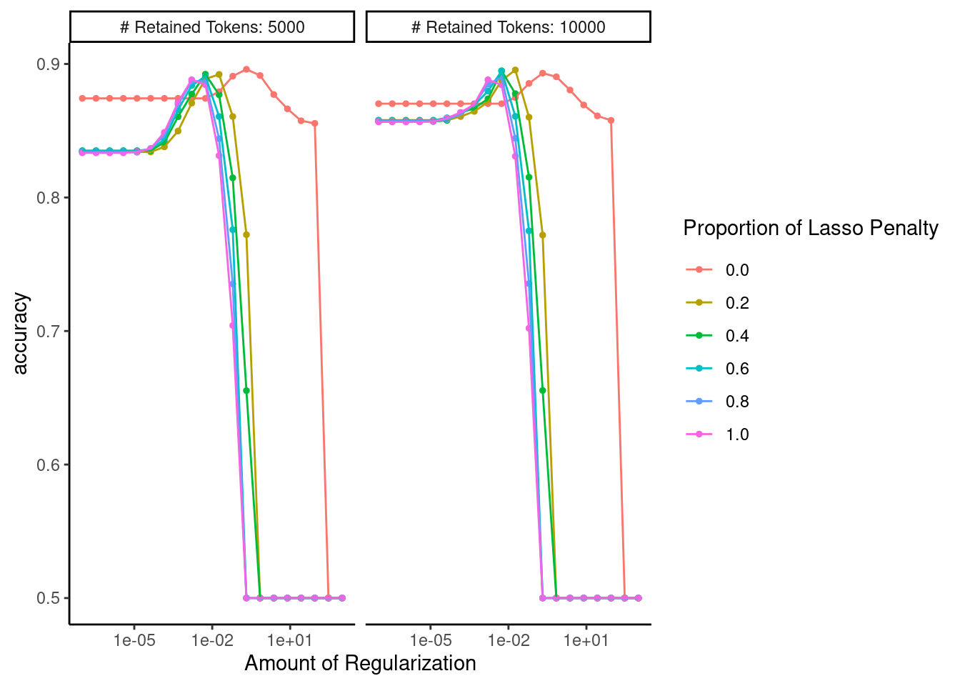
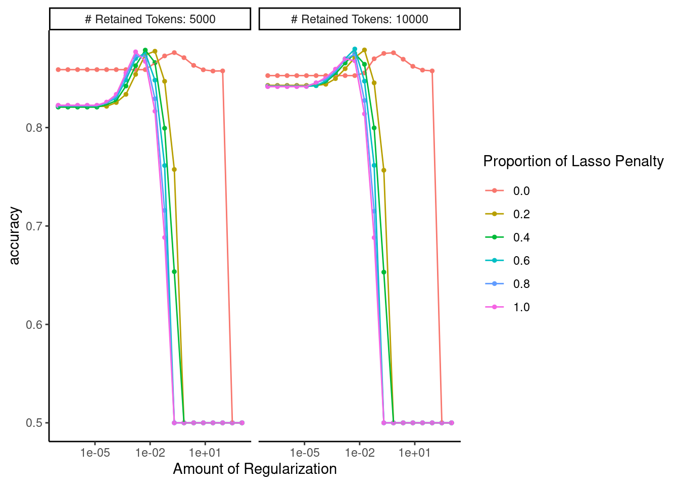
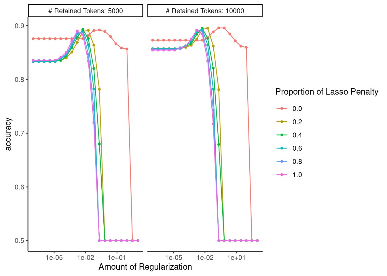
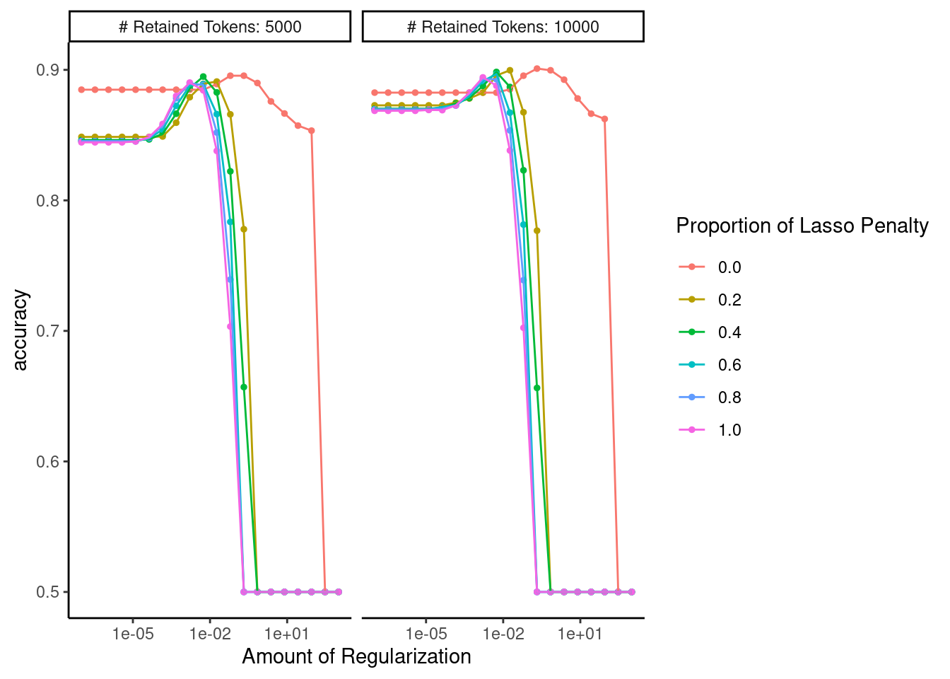
Confirm that the range of hyperparameters we considered was sufficient
autoplot(fits_ngrams)
Display performance of best configuration
Our best model yet!
show_best(fits_ngrams)
# A tibble: 5 × 9
  penalty mixture max_tokens .metric  .estimator  mean     n std_err
    <dbl>   <dbl>      <int> <chr>    <chr>      <dbl> <int>   <dbl>
1 0.207       0        10000 accuracy binary     0.901     1      NA
2 0.695       0        10000 accuracy binary     0.900     1      NA
3 0.0183      0.2      10000 accuracy binary     0.900     1      NA
4 0.00546     0.4      10000 accuracy binary     0.898     1      NA
5 0.00546     0.6      10000 accuracy binary     0.897     1      NA
  .config
  <chr>
1 Preprocessor2_Model013
2 Preprocessor2_Model014
3 Preprocessor2_Model031
4 Preprocessor2_Model050
5 Preprocessor2_Model070
12.8.6 Word Embeddings
BoW is an introductory approach for feature engineering.
As you have read, word embeddings are a common alternative that addresses some of the limitations of BoW. Word embeddings are also well-support in the tidyrecipes package.
Let’s switch gears away from document term matrices and BoW to word embeddings
You can find pre-trained word embeddings on the web
Below, we download and open pre-trained GloVe embeddings
I chose a smaller set of embeddings to ease computational cost
Wikipedia 2014 + Gigaword 5
6B tokens, 400K vocab, uncased, 50d
temp <-tempfile()options(timeout =max(300, getOption("timeout"))) # need more time to download big filedownload.file("https://nlp.stanford.edu/data/glove.6B.zip", temp)unzip(temp, files ="glove.6B.50d.txt")glove_embeddings <-read_delim(here::here("glove.6B.50d.txt"),delim =" ",col_names =FALSE)
Rows: 8 Columns: 51
── Column specification ────────────────────────────────────────────────────────
Delimiter: " "
chr  (1): X1
dbl (50): X2, X3, X4, X5, X6, X7, X8, X9, X10, X11, X12, X13, X14, X15, X16,...

ℹ Use `spec()` to retrieve the full column specification for this data.
ℹ Specify the column types or set `show_col_types = FALSE` to quiet this message.
Recipe for GloVe embedding. NOTES:
token = "words"
No need to filter tokens
New step is step_word_embeddings(text, embeddings = glove_embeddings)
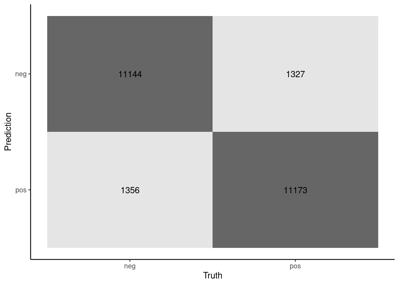
cm <-tibble(truth = feat_test$sentiment,estimate =predict(fit_final, feat_test)$.pred_class) |>conf_mat(truth, estimate)autoplot(cm, type ="heatmap")
And lets end by calculating Permutation feature importance scores in test set using DALEX
library(DALEX, exclude="explain")
Welcome to DALEX (version: 2.4.3).
Find examples and detailed introduction at: http://ema.drwhy.ai/
library(DALEXtra)
We are going to sample only a subset of the test set to keep the computational costs lower for this example.
set.seed(12345)feat_subtest <- feat_test |>slice_sample(prop = .05) # 5% of data
Now we can get a df for the features (without the outcome) and a separate vector for the outcome.
x <- feat_subtest |>select(-sentiment)
For outcome, we need to convert to 0/1 (if classification), and then pull the vector out of the dataframe
y <- feat_subtest |>mutate(sentiment =if_else(sentiment =="pos", 1, 0)) |>pull(sentiment)
We also need a specific predictor function that will work with the DALEX package
predict_wrapper <-function(model, newdata) {predict(model, newdata, type ="prob") |>pull(.pred_pos)}
We will also need an explainer object based on our model and data
explain_test <-explain_tidymodels(fit_final, # our model object data = x, # df with features without outcomey = y, # outcome vector# our custom predictor functionpredict_function = predict_wrapper)
Preparation of a new explainer is initiated
  -> model label       :  model_fit  (  default  )
  -> data              :  1250  rows  10000  cols
  -> data              :  tibble converted into a data.frame
  -> target variable   :  1250  values
  -> predict function  :  predict_function
  -> predicted values  :  No value for predict function target column. (  default  )
  -> model_info        :  package parsnip , ver. 1.1.0.9004 , task classification (  default  )
  -> predicted values  :  numerical, min =  0.0003611459 , mean =  0.5143743 , max =  0.9999001
  -> residual function :  residual_function
  -> residuals         :  numerical, min =  0 , mean =  0 , max =  0
  A new explainer has been created!
Finally, we need to define a custom function for our performance metric as well
Reading and discussion only for both units. Discussion requires you!
Two weeks left!
next tuesday (lab on NLP)
next thursday (discussion on applications)
following tuesday (discussion on ethics/fairness)
following thursday (concepts final review; 50 minutes only)
Early start to final application assignment (assigned next thursday, April 25th) and due Wednesday, May 8th at 8pm
Concepts exam at lab time during finals period (Tuesday, May 7th, 11-12:15 in this room)
13.2 Single nominal variable
Our algorithms need features coded with numbers
How did we generally do this?
What about algorithms like random forest?
13.3 Single nominal variable Example
Current emotional state
angry, afraid, sad, excited, happy, calm
How represented with one-hot?
13.4 What about document of words (e.g., sentence rather than single word)
I watched a scary movie last night and couldn’t get to sleep because I was so afraid
I went out with my friends to a bar and slept poorly because I drank too much
How represented with bag of words?
binary, count, tf-idf
What are the problems with these approaches
relationships between features or similarity between full vector across observations
context/order
dimensionality
sparsity
13.5 N-grams vs. simple (1-gram) BOW
How different?
some context/order
but still no relationship/meaning or similarity
even higher dimesions
13.6 Linguistic Inquiry and Word Count (LIWC)
Tausczik, Y. R., & Pennebaker, J. W. (2010). The psychological meaning of words: LIWC and computerized text analysis methods. Journal of Language and Social Psychology, 29(1), 24–54. https://doi.org/
Meaningful features? (based on domain expertise)
Lower dimensional
Very limited breadth
- Can add domain specific dictionaries
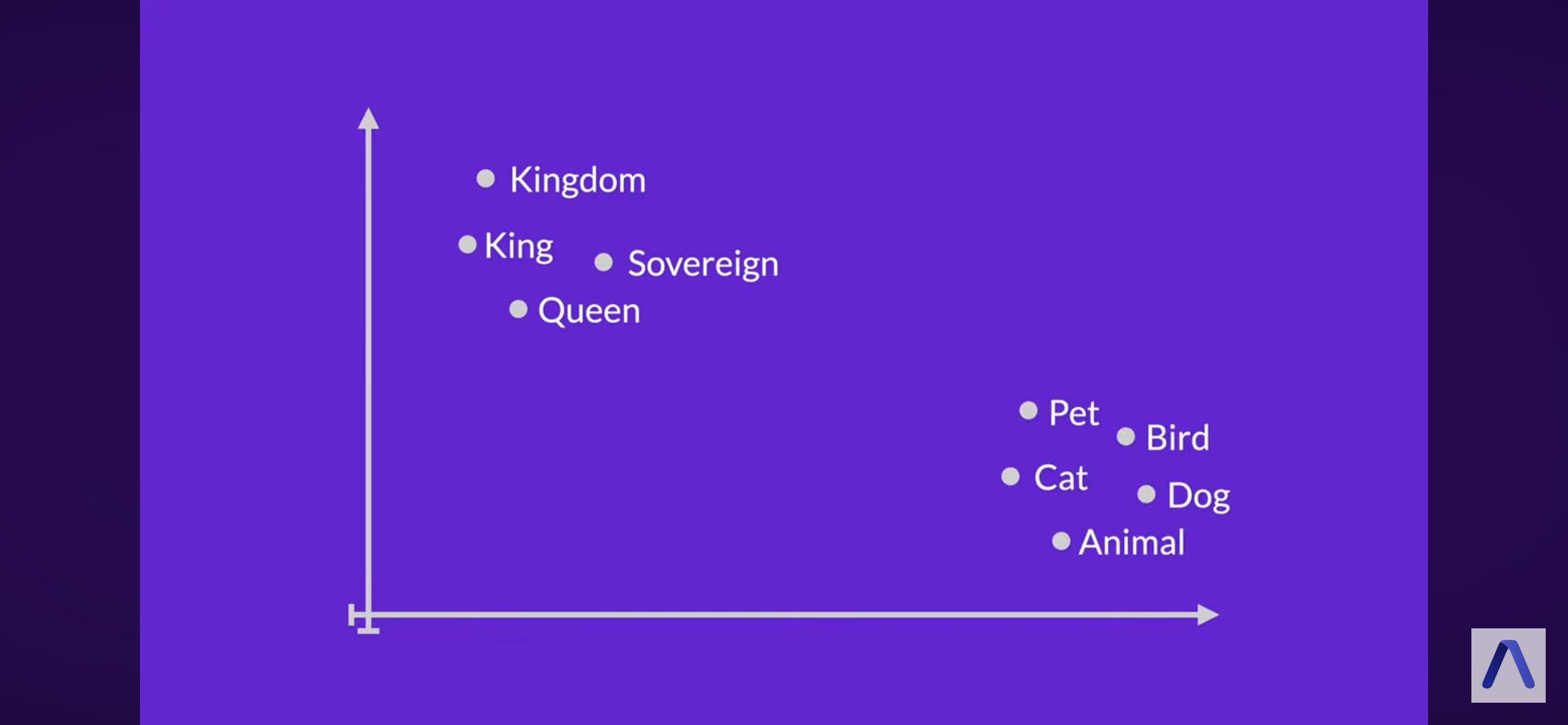
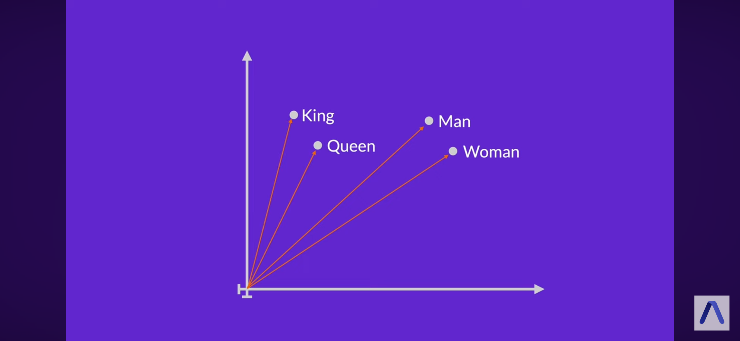
13.7 Word Embeddings
Encodes word meaning
Words that are similar get similar vectors
Meaning derived from context in various text corpora
Lower dimensional
Less sparse
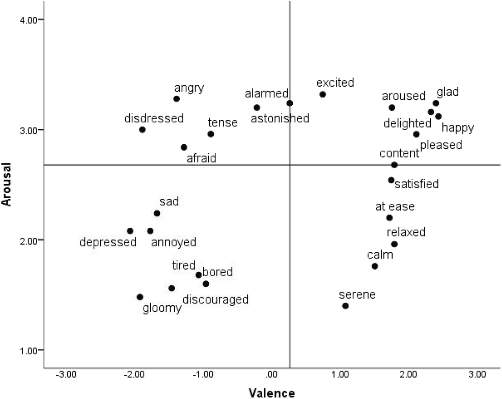
13.8 Examples
Affect Words
Two more general
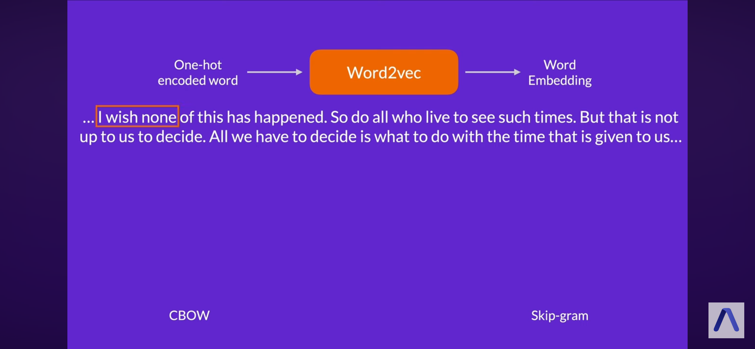
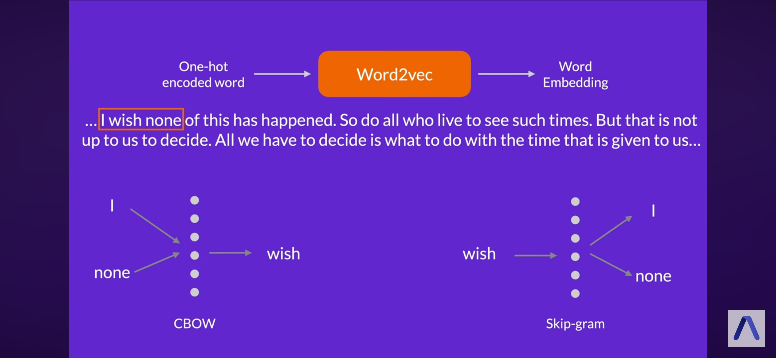
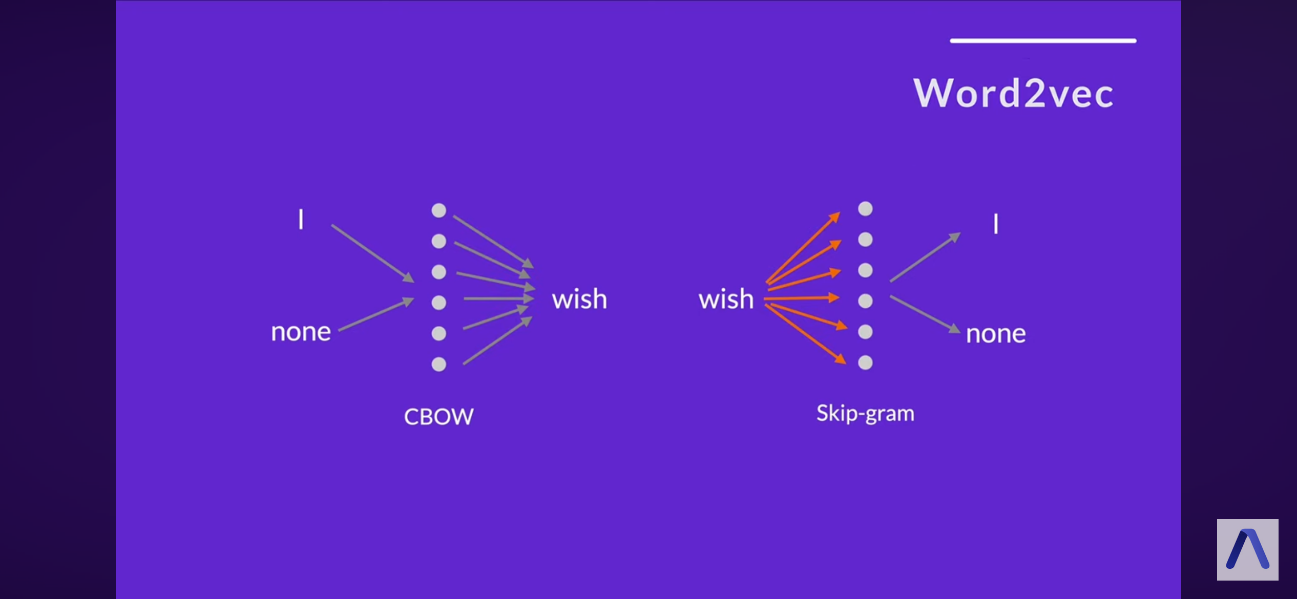
word2vec (google)
CBOW
skipgram
13.9 fasttext (facebook ai team)
n-grams (e.g., 3-6 character representations)
word vector is sum of its ngrams
can handle low frequecynor even novel wordsp
13.10 Other Methods
Other approaches
glove
elmo
BERT :w
Hvitfeldt, Emil, and Julia Silge. 2022. Supervised MachineLearning for TextAnalysis in R. https://smltar.com/.
Silge, Julia, and David Robinson. 2017. Text Mining with R: A Tidy Approach. 1rst ed. Beijing; Boston: O’Reilly Media.
Wickham, Hadley, Çetinkaya-Rundel Mine, and Garrett Grolemund. 2023. R for Data Science: Visualize, Model, Transform, and Import Data. 2nd ed. https://r4ds.hadley.nz/.